visreg tries to set up pleasant-looking default options, but everything can be tailored to user specifications. For the plots below, we work from this general model:
Turning on/off plot components
By default, visreg includes the fitted line, confidence bands, and partial residuals, but the residuals and the bands can be turned off:
visreg(fit, "Wind", band = FALSE)
visreg(fit, "Wind", partial = FALSE)
visreg(fit, "Wind", partial = FALSE, rug = TRUE)
Jittering
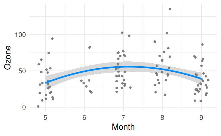
If there are many ties in a numeric variable x, jittering can be helpful way to avoid overplotting. Compare the following two plots:
month_fit <- lm(Ozone ~ Solar.R + Wind + poly(Month, 2), data = airquality)
visreg(month_fit, "Month")
visreg(month_fit, "Month", jitter = TRUE)
Appearance of points, lines, and bands
Specifying col='red' won’t work, because visreg can’t know whether you’re trying to change the color of the line, the band, or the points. These options must be specified through separate parameter lists:
-
line: Controls the appearance of the fitted line -
fill: Controls the appearance of the confidence band -
points: Controls the appearance of the partial residuals
Each of these is passed along to the underlying ggplot2 geom (geom_line/geom_ribbon/geom_point for a continuous x, or geom_errorbar/geom_tile/geom_jitter for a factor x), so any parameter that geom accepts can be specified:

Generic plot options
visreg returns a gg object, so its appearance can be customized just like any other ggplot2 plot, by adding further components. Here’s an example that adds a title and re-labels the (log-transformed) y-axis:

Band width for factors
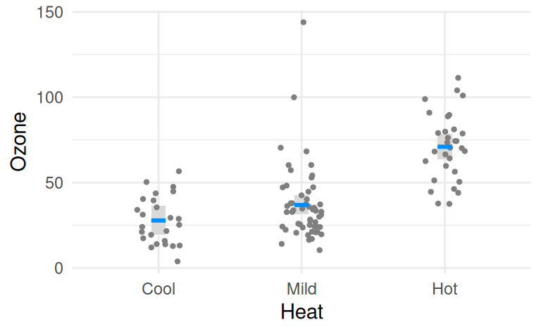
When x is a factor, the width of the confidence band (and its accompanying line) is controlled through the fill/line arguments’ width parameter:
fit <- lm(Ozone ~ Solar.R + Wind + Heat, data = airquality)
visreg(fit, "Heat", line = list(width = 0.98), fill = list(width = 0.98))
visreg(fit, "Heat", line = list(width = 0.1), fill = list(width = 0.1))
Subsetting the plot
Occasionally, you might want to plot only a subset of the levels or observations; you can use subset to accomplish this:

