Fit lasso penalized regression path for big data

Extend lasso model fitting to big data that cannot be loaded into memory. Fit solution paths for linear, logistic or Cox regression models penalized by lasso, ridge, or elastic-net over a grid of values for the regularization parameter lambda.

biglasso(
  X,
  y,
  row.idx = 1:nrow(X),
  penalty = c("lasso", "ridge", "enet"),
  family = c("gaussian", "binomial", "cox", "mgaussian"),
  alg.logistic = c("Newton", "MM"),
  screen = c("Adaptive", "SSR", "Hybrid", "None"),
  safe.thresh = 0,
  update.thresh = 1,
  ncores = 1,
  alpha = 1,
  lambda.min = ifelse(nrow(X) > ncol(X), 0.001, 0.05),
  nlambda = 100,
  lambda.log.scale = TRUE,
  lambda,
  eps = 1e-07,
  max.iter = 1000,
  dfmax = ncol(X) + 1,
  penalty.factor = rep(1, ncol(X)),
  warn = TRUE,
  output.time = FALSE,
  return.time = TRUE,
  verbose = FALSE
)

Arguments

X: The design matrix, without an intercept. It must be a double type bigmemory::big.matrix() object. The function standardizes the data and includes an intercept internally by default during the model fitting.
y: The response vector for family="gaussian" or family="binomial". For family="cox", y should be a two-column matrix with columns 'time' and 'status'. The latter is a binary variable, with '1' indicating death, and '0' indicating right censored. For family="mgaussin", y should be a n*m matrix where n is the sample size and m is the number of responses.
row.idx: The integer vector of row indices of X that used for fitting the model. 1:nrow(X) by default.
penalty: The penalty to be applied to the model. Either "lasso" (the default), "ridge", or "enet" (elastic net).
family: Either "gaussian", "binomial", "cox" or "mgaussian" depending on the response.
alg.logistic: The algorithm used in logistic regression. If "Newton" then the exact hessian is used (default); if "MM" then a majorization-minimization algorithm is used to set an upper-bound on the hessian matrix. This can be faster, particularly in data-larger-than-RAM case.
screen: The feature screening rule used at each lambda that discards features to speed up computation: "SSR" (default if penalty="ridge" or penalty="enet" )is the sequential strong rule; "Hybrid" is our newly proposed hybrid screening rules which combine the strong rule with a safe rule. "Adaptive" (default for penalty="lasso" without penalty.factor) is our newly proposed adaptive rules which reuse screening reference for multiple lambda values. Note that: (1) for linear regression with elastic net penalty, both "SSR" and "Hybrid" are applicable since version 1.3-0; (2) only "SSR" is applicable to elastic-net-penalized logistic regression or cox regression; (3) active set cycling strategy is incorporated with these screening rules.
safe.thresh: the threshold value between 0 and 1 that controls when to stop safe test. For example, 0.01 means to stop safe test at next lambda iteration if the number of features rejected by safe test at current lambda iteration is not larger than 1\ to always turn off safe test, whereas 0 (default) means to turn off safe test if the number of features rejected by safe test is 0 at current lambda.
update.thresh: the non negative threshold value that controls how often to update the reference of safe rules for "Adaptive" methods. Smaller value means updating more often.
ncores: The number of OpenMP threads used for parallel computing.
alpha: The elastic-net mixing parameter that controls the relative contribution from the lasso (l1) and the ridge (l2) penalty. The penalty is defined as $$ \alpha||\beta||_1 + (1-\alpha)/2||\beta||_2^2.$$ alpha=1 is the lasso penalty, alpha=0 the ridge penalty, alpha in between 0 and 1 is the elastic-net ("enet") penalty.
lambda.min: The smallest value for lambda, as a fraction of lambda.max. Default is .001 if the number of observations is larger than the number of covariates and .05 otherwise.
nlambda: The number of lambda values. Default is 100.
lambda.log.scale: Whether compute the grid values of lambda on log scale (default) or linear scale.
lambda: A user-specified sequence of lambda values. By default, a sequence of values of length nlambda is computed, equally spaced on the log scale.
eps: Convergence threshold for inner coordinate descent. The algorithm iterates until the maximum change in the objective after any coefficient update is less than eps times the null deviance. Default value is 1e-7.
max.iter: Maximum number of iterations. Default is 1000.
dfmax: Upper bound for the number of nonzero coefficients. Default is no upper bound. However, for large data sets, computational burden may be heavy for models with a large number of nonzero coefficients.
penalty.factor: A multiplicative factor for the penalty applied to each coefficient. If supplied, penalty.factor must be a numeric vector of length equal to the number of columns of X. The purpose of penalty.factor is to apply differential penalization if some coefficients are thought to be more likely than others to be in the model. Current package doesn't allow unpenalized coefficients. That ispenalty.factor cannot be 0. penalty.factor is only supported for "SSR" screen.
warn: Return warning messages for failures to converge and model saturation? Default is TRUE.
output.time: Whether to print out the start and end time of the model fitting. Default is FALSE.
return.time: Whether to return the computing time of the model fitting. Default is TRUE.
verbose: Whether to output the timing of each lambda iteration. Default is FALSE.

Value

An object with S3 class "biglasso" for "gaussian", "binomial", "cox" families, or an object with S3 class "mbiglasso" for "mgaussian" family, with following variables.

beta: The fitted matrix of coefficients, store in sparse matrix representation. The number of rows is equal to the number of coefficients, whereas the number of columns is equal to nlambda. For "mgaussian" family with m responses, it is a list of m such matrices.
iter: A vector of length nlambda containing the number of iterations until convergence at each value of lambda.
lambda: The sequence of regularization parameter values in the path.
penalty: Same as above.
family: Same as above.
alpha: Same as above.
loss: A vector containing either the residual sum of squares (for "gaussian", "mgaussian") or negative log-likelihood (for "binomial", "cox") of the fitted model at each value of lambda.
penalty.factor: Same as above.
n: The number of observations used in the model fitting. It's equal to length(row.idx).
center: The sample mean vector of the variables, i.e., column mean of the sub-matrix of X used for model fitting.
scale: The sample standard deviation of the variables, i.e., column standard deviation of the sub-matrix of X used for model fitting.
y: The response vector used in the model fitting. Depending on row.idx, it could be a subset of the raw input of the response vector y.
screen: Same as above.
col.idx: The indices of features that have 'scale' value greater than 1e-6. Features with 'scale' less than 1e-6 are removed from model fitting.
rejections: The number of features rejected at each value of lambda.
safe_rejections: The number of features rejected by safe rules at each value of lambda.

Details

The objective function for linear regression or multiple responses linear regression (family = "gaussian" or family = "mgaussian") is $$\frac{1}{2n}\textrm{RSS} + \lambda*\textrm{penalty},$$ where for family = "mgaussian"), a group-lasso type penalty is applied. For logistic regression (family = "binomial") it is $$-\frac{1}{n} loglike + \lambda*\textrm{penalty},$$, for cox regression, breslow approximation for ties is applied.

Several advanced feature screening rules are implemented. For lasso-penalized linear regression, all the options of screen are applicable. Our proposal adaptive rule - "Adaptive" - achieves highest speedup so it's the recommended one, especially for ultrahigh-dimensional large-scale data sets. For cox regression and/or the elastic net penalty, only "SSR" is applicable for now. More efficient rules are under development.

Author

Yaohui Zeng, Chuyi Wang and Patrick Breheny

Examples

## Linear regression
data(colon)
X <- colon$X
y <- colon$y
X.bm <- as.big.matrix(X)
# lasso, default
par(mfrow=c(1,2))
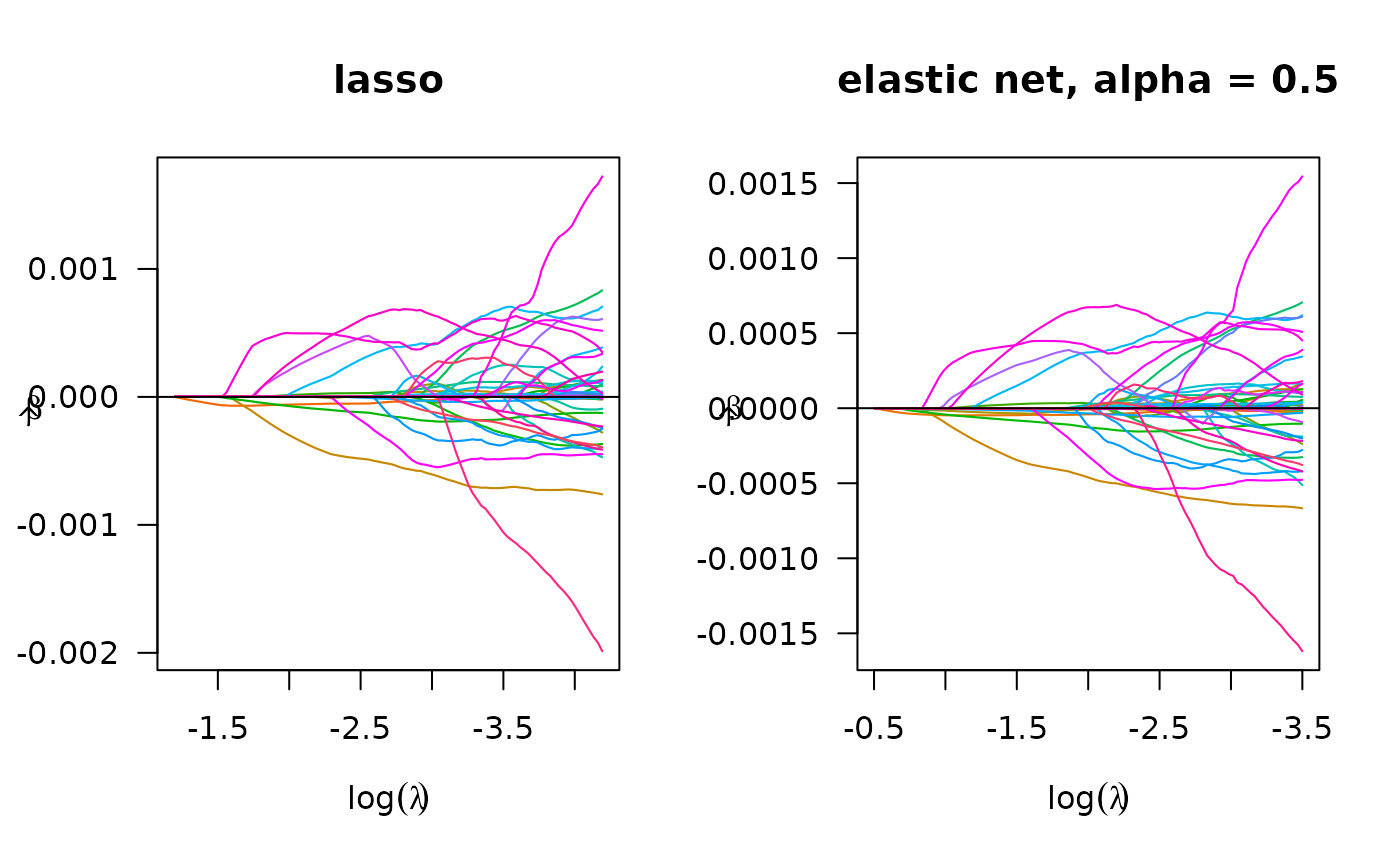
fit.lasso <- biglasso(X.bm, y, family = 'gaussian')
plot(fit.lasso, log.l = TRUE, main = 'lasso')
# elastic net
fit.enet <- biglasso(X.bm, y, penalty = 'enet', alpha = 0.5, family = 'gaussian')
plot(fit.enet, log.l = TRUE, main = 'elastic net, alpha = 0.5')


## Logistic regression
data(colon)
X <- colon$X
y <- colon$y
X.bm <- as.big.matrix(X)
# lasso, default
par(mfrow = c(1, 2))
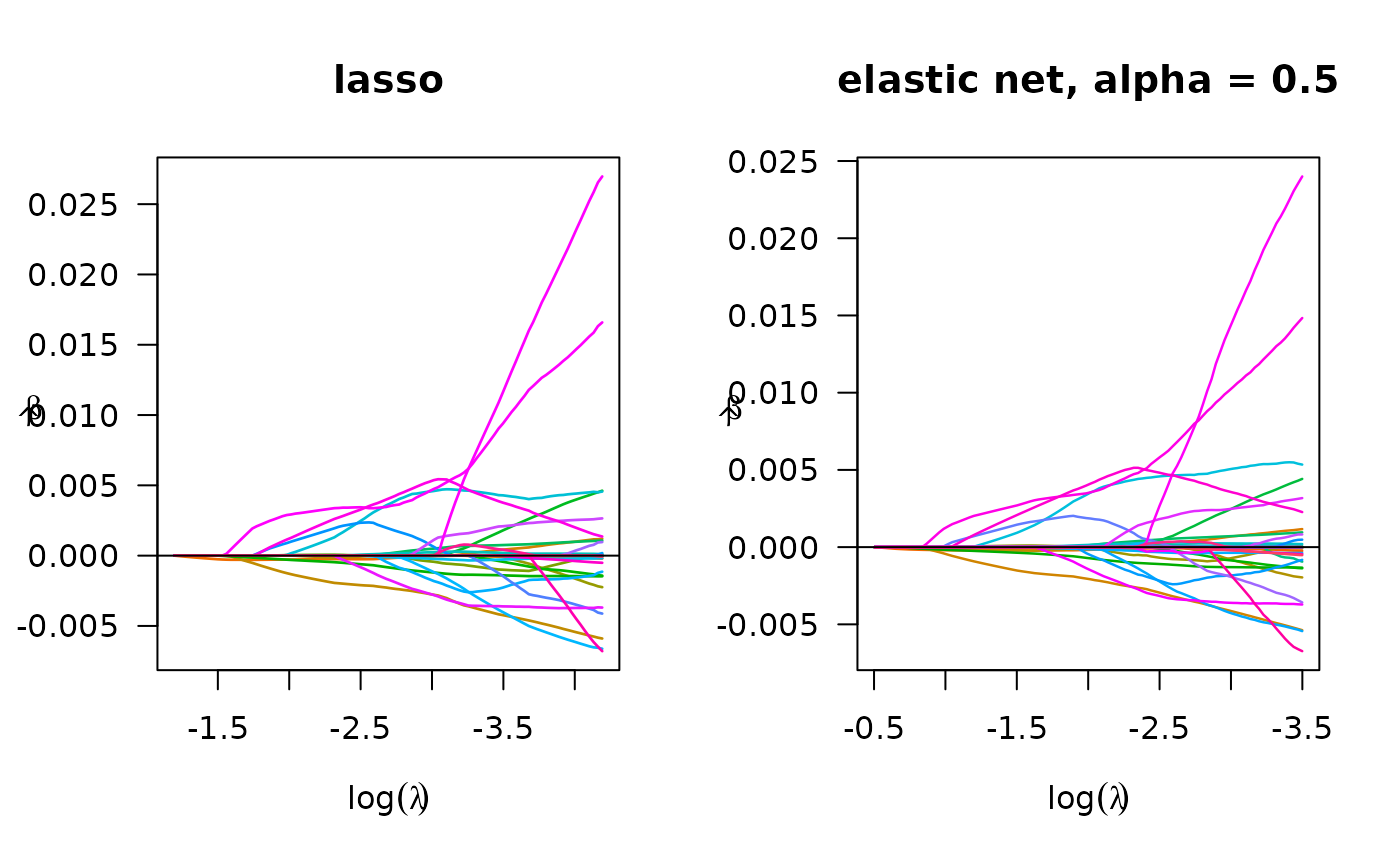
fit.bin.lasso <- biglasso(X.bm, y, penalty = 'lasso', family = "binomial")
plot(fit.bin.lasso, log.l = TRUE, main = 'lasso')
# elastic net
fit.bin.enet <- biglasso(X.bm, y, penalty = 'enet', alpha = 0.5, family = "binomial")
plot(fit.bin.enet, log.l = TRUE, main = 'elastic net, alpha = 0.5')


## Cox regression
set.seed(10101)
N <- 1000; p <- 30; nzc <- p/3
X <- matrix(rnorm(N * p), N, p)
beta <- rnorm(nzc)
fx <- X[, seq(nzc)] %*% beta/3
hx <- exp(fx)
ty <- rexp(N, hx)
tcens <- rbinom(n = N, prob = 0.3, size = 1)  # censoring indicator
y <- cbind(time = ty, status = 1 - tcens)  # y <- Surv(ty, 1 - tcens) with library(survival)
X.bm <- as.big.matrix(X)
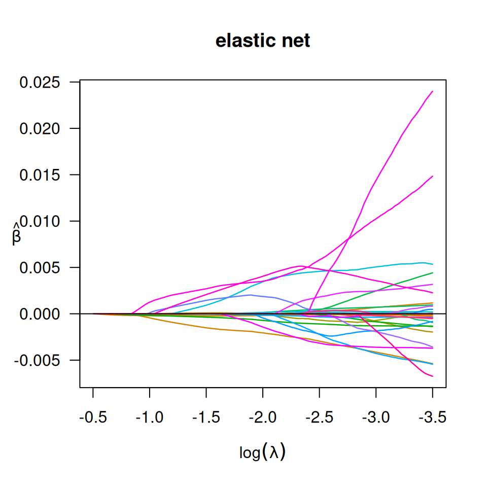
fit <- biglasso(X.bm, y, family = "cox")
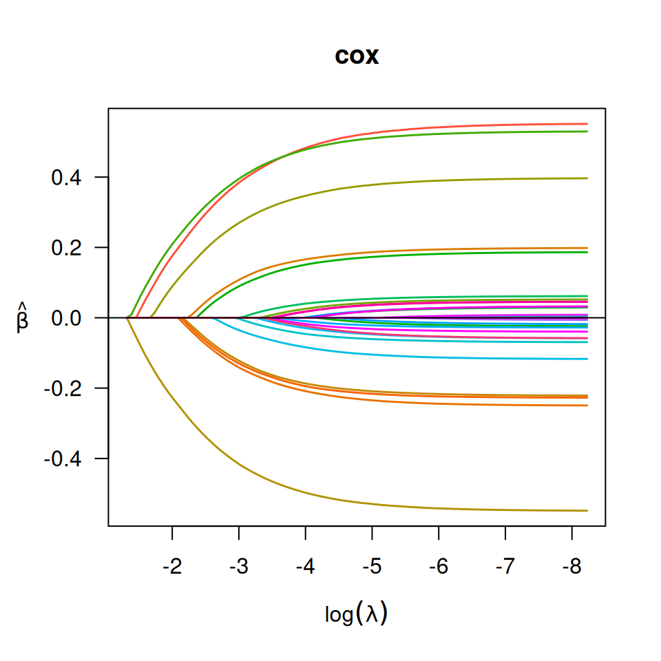
plot(fit, main = "cox")

## Multiple responses linear regression
set.seed(10101)
n=300; p=300; m=5; s=10; b=1
x = matrix(rnorm(n * p), n, p)
beta = matrix(seq(from=-b,to=b,length.out=s*m),s,m)
y = x[,1:s] %*% beta + matrix(rnorm(n*m,0,1),n,m)
x.bm = as.big.matrix(x)
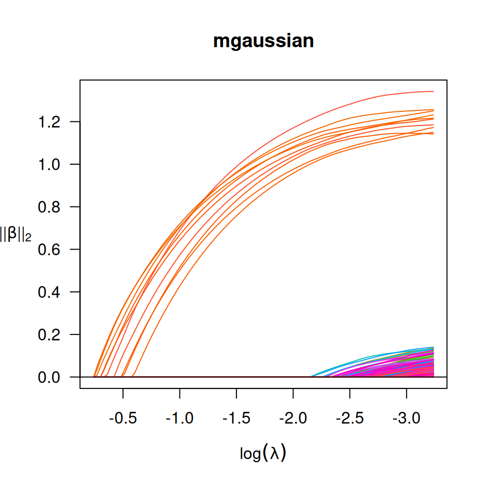
fit = biglasso(x.bm, y, family = "mgaussian")
plot(fit, main = "mgaussian")

References

Zeng Y and Breheny P. (2021) The biglasso Package: A Memory- and Computation- Efficient Solver for Lasso Model Fitting with Big Data in R. R Journal, 12: 6-19. doi:10.32614/RJ-2021-001