Small Data
Linear regression
library(biglasso)
#> Loading required package: bigmemory
#> Loading required package: Matrix
#> Loading required package: ncvreg

data(colon)
X <- colon$X
y <- colon$y
dim(X)
#> [1]   62 2000
X[1:5, 1:5]
#>   Hsa.3004 Hsa.13491 Hsa.13491.1 Hsa.37254 Hsa.541
#> t  8589.42   5468.24     4263.41   4064.94 1997.89
#> n  9164.25   6719.53     4883.45   3718.16 2015.22
#> t  3825.71   6970.36     5369.97   4705.65 1166.55
#> n  6246.45   7823.53     5955.84   3975.56 2002.61
#> t  3230.33   3694.45     3400.74   3463.59 2181.42
# convert X to a big.matrix object
# X.bm is a pointer to the data matrix
X.bm <- as.big.matrix(X)
str(X.bm)
#> Formal class 'big.matrix' [package "bigmemory"] with 1 slot
#>   ..@ address:<pointer: 0x5584433375d0>
dim(X.bm)
#> [1]   62 2000
Note that this is the same as X[1:5, 1:5]:
X.bm[1:5, 1:5]
#>   Hsa.3004 Hsa.13491 Hsa.13491.1 Hsa.37254 Hsa.541
#> t  8589.42   5468.24     4263.41   4064.94 1997.89
#> n  9164.25   6719.53     4883.45   3718.16 2015.22
#> t  3825.71   6970.36     5369.97   4705.65 1166.55
#> n  6246.45   7823.53     5955.84   3975.56 2002.61
#> t  3230.33   3694.45     3400.74   3463.59 2181.42
Cross-Validation
To run cross-validation, use cv.biglasso():
cvfit <- cv.biglasso(X.bm, y, seed = 1234, nfolds = 10)After cross-validation, a few things we can do:
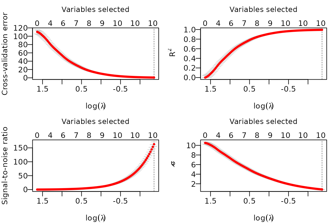
- plot the cross-validation plots:

- Summarize CV object:
summary(cvfit)
#> lasso-penalized linear regression with n=62, p=2000
#> At minimum cross-validation error (lambda=0.0386):
#> -------------------------------------------------
#>   Nonzero coefficients: 27
#>   Cross-validation error (deviance): 0.14
#>   R-squared: 0.40
#>   Signal-to-noise ratio: 0.66
#> Scale estimate (sigma): 0.371- Extract non-zero coefficients at the optimal \lambda value:
coef(cvfit)[which(coef(cvfit) != 0), ]
#>   (Intercept)      Hsa.8147     Hsa.43279     Hsa.36689      Hsa.3152
#>  6.882526e-01 -5.704059e-07 -2.748858e-08 -6.967419e-04  4.940698e-05
#>     Hsa.36665     Hsa.692.2      Hsa.1272       Hsa.166     Hsa.31801
#>  1.297733e-05 -1.878545e-04 -1.808689e-04  3.717512e-04  1.119437e-04
#>      Hsa.3648      Hsa.1047     Hsa.13628      Hsa.3016      Hsa.5392
#>  1.508691e-04  6.557284e-07  6.519466e-05  2.479566e-05  5.741251e-04
#>      Hsa.1832      Hsa.1464     Hsa.12241     Hsa.44244      Hsa.9246
#> -4.052627e-05  1.821951e-05 -1.912212e-04 -3.369856e-04 -1.582765e-06
#>     Hsa.41159     Hsa.33268      Hsa.6814      Hsa.1660       Hsa.404
#>  3.974870e-04 -4.911208e-04  5.639023e-04  5.171245e-04 -5.208537e-05
#>     Hsa.43331      Hsa.1491   Hsa.41098.1
#> -6.853944e-04  2.977285e-04 -1.748628e-04
Logistic Regression
data(Heart)
X <- Heart$X
y <- Heart$y
X.bm <- as.big.matrix(X)
fit <- biglasso(X.bm, y, family = "binomial")
plot(fit)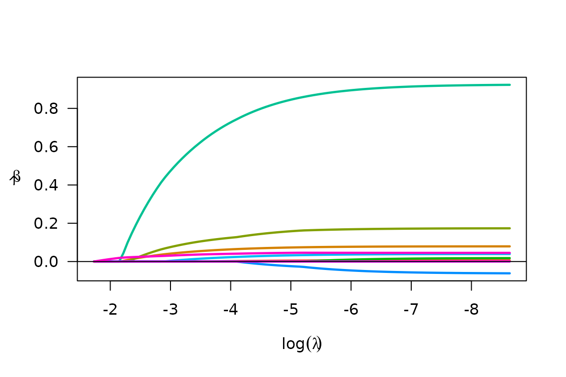
Cox Regression
library(survival)
#>
#> Attaching package: 'survival'
#> The following object is masked _by_ '.GlobalEnv':
#>
#>     colon
X <- heart[, 4:7]
y <- Surv(heart$stop - heart$start, heart$event)
X.bm <- as.big.matrix(X)
#> Warning in as.big.matrix(X): Coercing data.frame to matrix via factor level
#> numberings.
fit <- biglasso(X.bm, y, family = "cox")
plot(fit)
Multiple response Linear Regression (multitask learning)
set.seed(10101)
n <- 300
p <- 300
m <- 5
s <- 10
b <- 1
x <- matrix(rnorm(n * p), n, p)
beta <- matrix(seq(from = -b, to = b, length.out = s * m), s, m)
y <- x[, 1:s] %*% beta + matrix(rnorm(n * m, 0, 1), n, m)
x.bm <- as.big.matrix(x)
fit <- biglasso(x.bm, y, family = "mgaussian")
plot(fit)
Big Data
When the raw data file is very large, it’s better to convert the raw
data file into a file-backed big.matrix by using a file
cache. We can call function setupX, which reads the raw
data file and creates a backing file (.bin) and a descriptor file
(.desc) for the raw data matrix:
# The data has 200 observations, 600 features, and 10 non-zero coefficients.
# This is not actually very big, but vignettes in R are supposed to render
# quickly, so we'll have to pretend that this can't fit in memory.
# Much larger data can be handled in the same way.
if (!file.exists("BigX.bin")) {
  X <- matrix(rnorm(1000 * 5000), 1000, 5000)
  beta <- c(-5:5)
  y <- as.numeric(X[, 1:11] %*% beta)
  write.csv(X, "BigX.csv", row.names = FALSE)
  write.csv(y, "y.csv", row.names = FALSE)
  X.bm <- setupX("BigX.csv", header = TRUE)
}
#> Reading data from file, and creating file-backed big.matrix...
#> This should take a while if the data is very large...
#> Start time:  2026-08-27 19:53:32
#> End time:  2026-08-27 19:53:33
#> DONE!
#>
#> Note: This function needs to be called only one time to create two backing
#>       files (.bin, .desc) in current dir. Once done, the data can be
#>       'loaded' using function 'attach.big.matrix'. See details in doc.
It’s important to note that the above operation is only a one-time
execution. Once done, the data can be retrieved seamlessly by attaching
its descriptor file (.desc) in any new R session:
rm(list = c("X", "X.bm", "y")) # Pretend starting a new session
X.bm <- attach.big.matrix("BigX.desc")
y <- read.csv("y.csv")[, 1]
This is very appealing for big data analysis in that we don’t need to “read” the raw data again in a R session, which would be very time-consuming. The code below again fits a lasso-penalized linear model, and runs 10-fold cross-validation:
system.time({
  fit <- biglasso(X.bm, y)
})
#>    user  system elapsed
#>   0.192   0.001   0.193
plot(fit)
For large data sets, it is often convenient to run cross validation in parallel (you can certainly use more cores on your machine, but CRAN vignettes are only allowed to use 2):
cvfit <- cv.biglasso(X.bm, y, seed = 1234, ncores = 2, nfolds = 10)