grpreg fits models that fall into the penalized
likelihood framework. Rather than estimating \boldsymbol{\beta} by maximizing the
likelihood, in this framework we estimate \boldsymbol{\beta} by minimizing the
objective function
Q(\boldsymbol{\beta}|\mathbf{X}, \mathbf{y}) =
\frac{1}{n}L(\boldsymbol{\beta}|\mathbf{X},\mathbf{y}) +
P_\lambda(\boldsymbol{\beta}),
where the loss function L(\boldsymbol{\beta}|\mathbf{X},\mathbf{y})
is the negative log-likelihood (2 times
this quantity is known as the deviance), P_\lambda(\boldsymbol{\beta}) is the penalty,
and \lambda is a regularization
parameter that controls the tradeoff between the two components. This
article describes the different loss models available in
grpreg; see penalties for more
information on the different penalties available.
Gaussian (linear regression)
In linear regression, the loss function is simply the squared error loss: L(\boldsymbol{\beta}|\mathbf{X},\mathbf{y}) = \frac{1}{2} \lVert\mathbf{y}-\mathbf{X}\boldsymbol{\beta}\rVert_2^2; this is proportional to the negative log-likelihood for a model where y follows a Gaussian distribution with constant variance and mean equal to \mathbf{X}\boldsymbol{\beta}.
To fit a penalized linear regression model with
grpreg:
fit <- grpreg(X, y, group)Binomial (logistic regression)
In logistic regression, the loss function is: L(\boldsymbol{\beta}|\mathbf{X},\mathbf{y}) = -\sum_{i:y_i=1}\log\hat{\pi}_i - \sum_{i:y_i=0}\log(1-\hat{\pi}_i); this is the negative log-likelihood for a binomial distribution with probabilities P(Y_i=1)=\hat{\pi}_i given by: \hat{\pi}_i = \frac{\exp(\eta_i)}{1+\eta_i}, where \boldsymbol{\eta}= \mathbf{X}\boldsymbol{\beta} denotes the linear predictors.
To fit a penalized logistic regression model with
grpreg:
fit <- grpreg(X, y, group, family='binomial')Poisson
In Poisson regression, the loss function is: L(\boldsymbol{\beta}|\mathbf{X},\mathbf{y}) = 2\sum_i \left\{y_i\log y_i - y_i\log \mu_i + mu_i - y_i\right\}; note that some of these terms are constant with respect to \mu_i and can therefore be ignored during optimization. Twice this loss is the deviance for a Poisson distribution Y_i \sim \text{Pois}(\hat{\mu}_i) with rate parameter given by: \hat{\mu}_i = \exp(\eta_i).
To fit a penalized Poisson regression model with
grpreg:
fit <- grpreg(X, y, group, family='poisson')Cox proportional hazards
The above models all fall into the category of distributions known as
exponential families (hence the family) argument.
grpreg also allows users to fit Cox proportional hazards
models, although these models fall outside this framework and are
therefore fit using a different function, grpsurv. In Cox
regression, the negative log of the partial likelihood is
L(\boldsymbol{\beta}|\mathbf{X},\mathbf{y}) = -2\sum_{j=1}^{m} d_j
\eta_j + 2\sum_{j=1}^{m} d_j \log\left\{\sum_{i \in R_j}
\exp(\eta_i)\right\},
where t_1 < t_2 < \ldots <
t_m denotes an increasing list of unique failure times indexed by
j and R_j denotes the set of observations still at
risk at time t_j, known as the risk
set.
The Lung data (see ?Lung for more details)
provides an example of time-to-event data that can be used with Cox
regression. Loading this data set into R,
data(Lung)
X <- Lung$X
y <- Lung$y
group <- Lung$group
To fit a penalized Cox regression model,
fit <- grpsurv(X, y, group)As before, you can call plot, coef,
predict, etc. on fit:
coef(fit, lambda=0.1)
#        trt     karno1     karno2     karno3  diagtime1  diagtime2       age1
#  0.0000000 -4.6535992  0.4641241 -0.3283532  0.0000000  0.0000000  0.0000000
#       age2       age3      prior   squamous      small      adeno      large
#  0.0000000  0.0000000  0.0000000 -0.2613796  0.1320625  0.2666665 -0.1424394
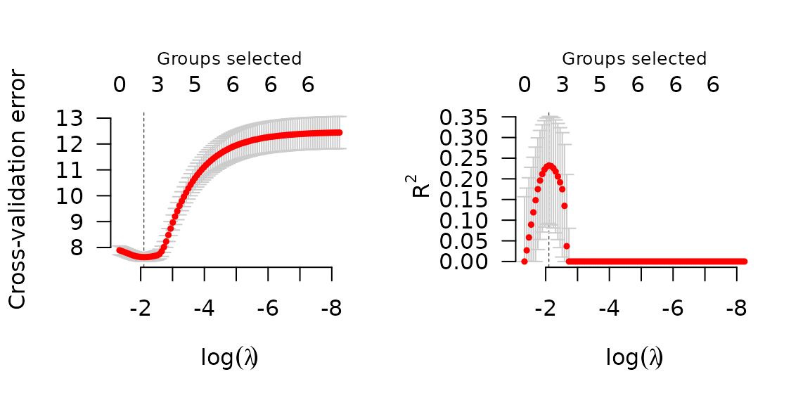
Cross-validation is similar:
set.seed(1)
cvfit <- cv.grpsurv(X, y, group)
par(mfrow=c(1,2))
plot(cvfit, type='cve')
plot(cvfit, type='rsq')
In addition to the quantities like coefficients and number of nonzero
coefficients that predict returns for other types of
models, predict() for an grpsurv object can
also estimate the baseline hazard (using the Kalbfleish-Prentice method)
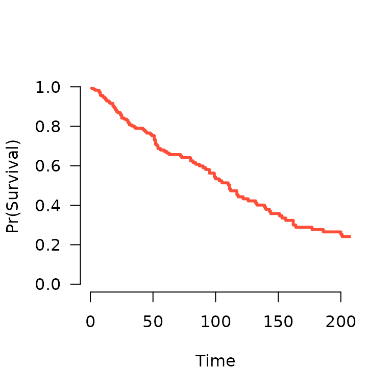
and therefore, the survival function. A method to plot the resulting
function is also available:
S <- predict(fit, X[1,], type='survival', lambda=0.02)
S(365)   # Estiamted survival at 1 year
# [1] 0.09995821
plot(S, xlim=c(0,200))
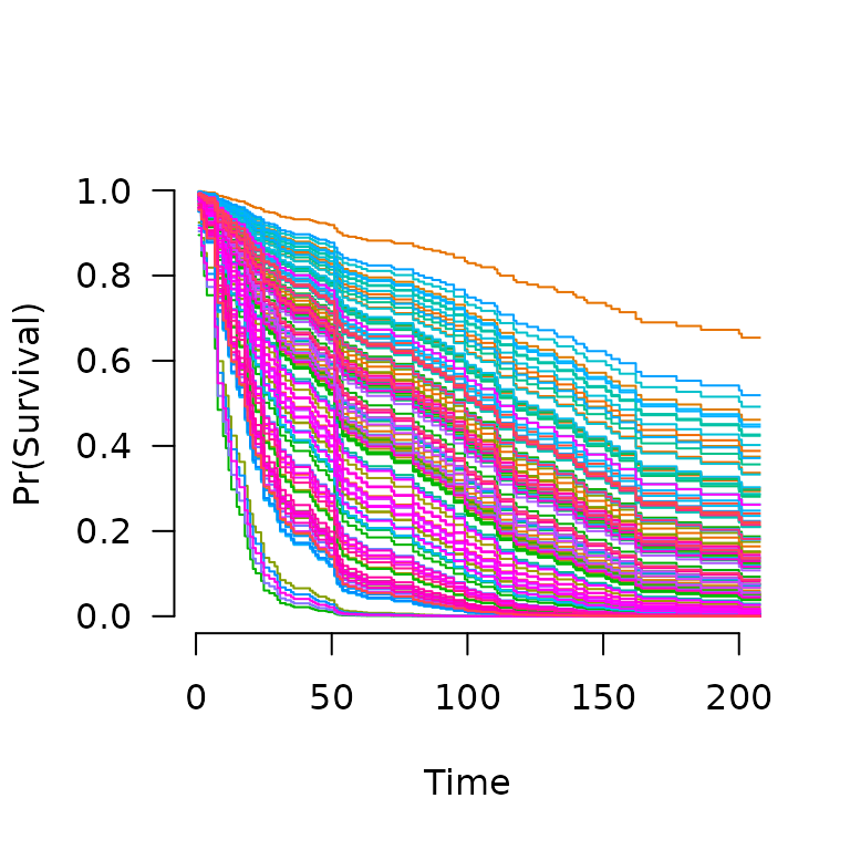
When multiple subjects are involved in the prediction:
S <- predict(fit, X, type='survival', lambda=0.02)
S[[1]](365)  # Estimated survival at 1 year for subject 1
# [1] 0.09995821
S[[2]](365)  # Estimated survival at 1 year for subject 2
# [1] 0.142846
plot(S, xlim=c(0,200))