Penalties

ncvreg fits models that fall into the penalized likelihood framework. Rather than estimating \boldsymbol{\beta} by maximizing the likelihood, in this framework we estimate \boldsymbol{\beta} by minimizing the objective function

Q(\boldsymbol{\beta}|\mathbf{X}, \mathbf{y}) = L(\boldsymbol{\beta}|\mathbf{X},\mathbf{y})+ P_\lambda(\boldsymbol{\beta}),

where L(\boldsymbol{\beta}|\mathbf{X},\mathbf{y}) is the loss (deviance) and P_\lambda(\boldsymbol{\beta}) is the penalty. This article describes the different penalties available in ncvreg; see models for more information on the different loss functions available. Throughout, linear regression and the Prostate data set is used

data(Prostate)
x <- Prostate$X
y <- Prostate$y

MCP

This is the default penalty in ncvreg.

P(\beta; \lambda, \gamma) = \begin{cases} \lambda|\beta|-\frac{\beta^2}{2\gamma}, & \text{if } |\beta| \leq \gamma\lambda\\ \frac{1}{2} \gamma\lambda^2, & \text{if } |\beta| > \gamma\lambda \end{cases}

for \gamma> 1, or more compactly,

P(\beta;\lambda, \gamma) = \lambda\int_0^{|\beta|} (1-t/(\gamma\lambda))_+ dt.

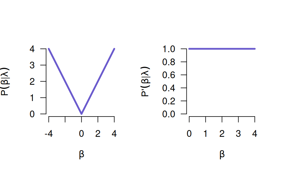
A plot of the MCP (penalty on left, derivative on right):

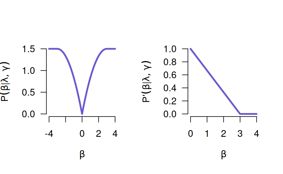
The MCP starts out by applying the same rate of penalization as the lasso, then smoothly relaxes the rate down to zero as the absolute value of the coefficient increases.

The following figure illustrates the effect of changing \gamma:

par(mfrow = c(1,3))
fit <- ncvreg(x, y, gamma = 1.5)
plot(fit, main = expression(paste(gamma, "=", 1.5)))
fit <- ncvreg(x, y)
plot(fit, main = expression(paste(gamma, "=", 3)))
fit <- ncvreg(x, y, gamma = 10)
plot(fit, main = expression(paste(gamma, "=", 10)))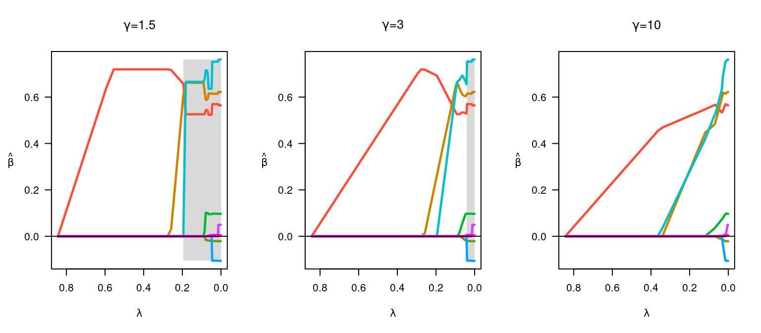

At smaller \gamma values, the estimates transition rapidly from 0 to their unpenalized solutions; this transition happens more slowly and gradually at larger \gamma values. Note that one consquence of these rapid transitions at low \gamma values is that the solutions are less stable (the gray region depicting the region of the solution path that is not locally convex is larger).

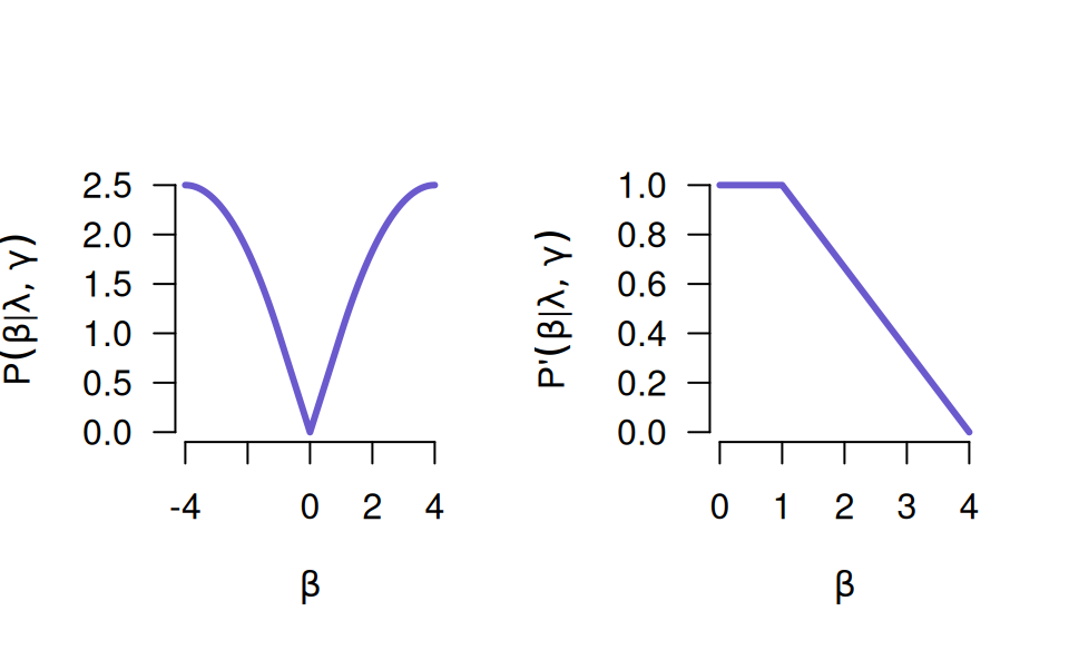
SCAD

The SCAD penalty is similar, except it does not immediately relax the penalty.

P(\beta; \lambda, \gamma) = \begin{cases} \lambda|\beta| & \text{if } |\beta| \leq \lambda, \\ \frac{2\gamma\lambda|\beta|-\beta^2-\lambda^2}{2(\gamma-1)} & \text{if } \lambda< |\beta| < \gamma\lambda, \\ \frac{\lambda^2(\gamma+1)}{2} & \text{if } |\beta| \geq \gamma\lambda, \end{cases}

or more compactly,

P(\beta; \lambda, \gamma) = \lambda\int_0^{|\beta|} \min\{1,(\gamma-t/\lambda)_+/(\gamma-1)\}dt.

Lasso

P(\beta; \lambda) = \lambda\left\lvert\beta\right\rvert

par(mfrow = c(1,3))
fit <- ncvreg(x, y)
plot(fit, main = "MCP")
fit <- ncvreg(x, y, penalty = "SCAD")
plot(fit, main = "SCAD")
fit <- ncvreg(x, y, penalty = "lasso")
plot(fit, main = "Lasso")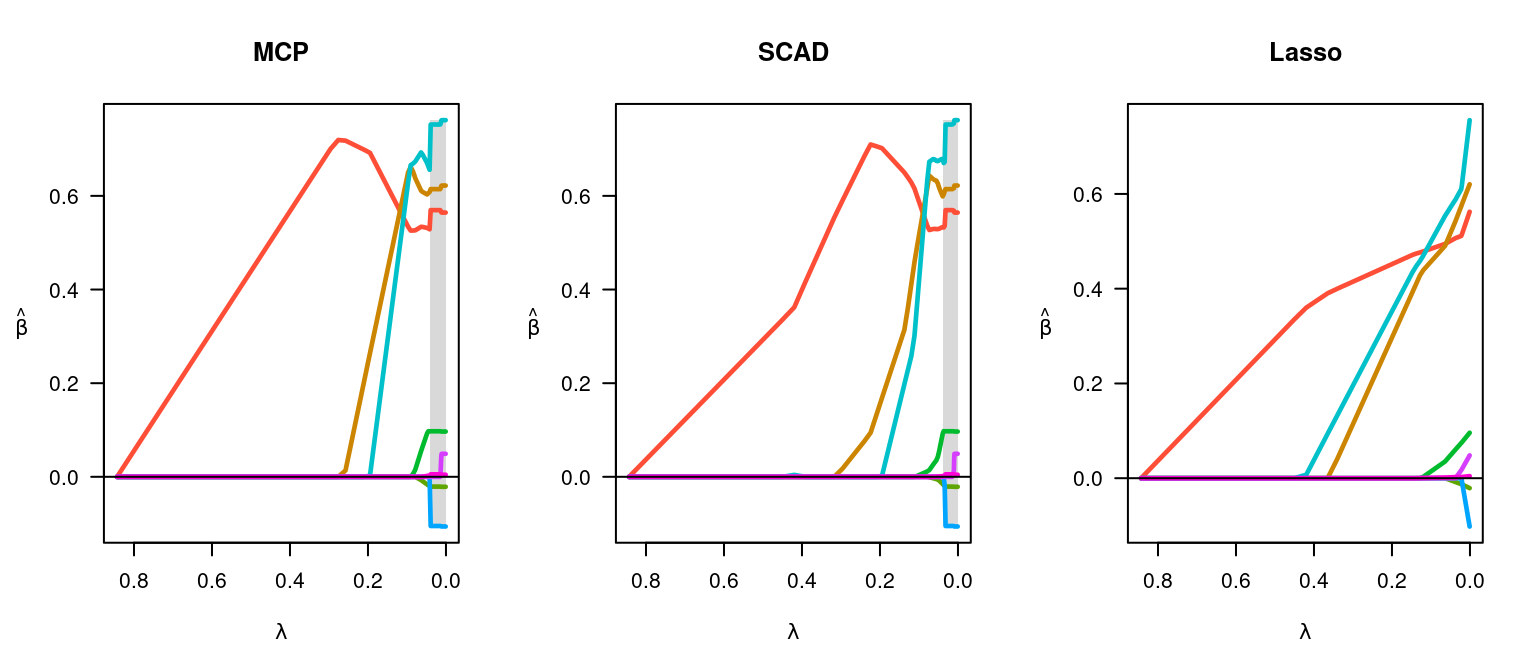

Elastic Net and MNet

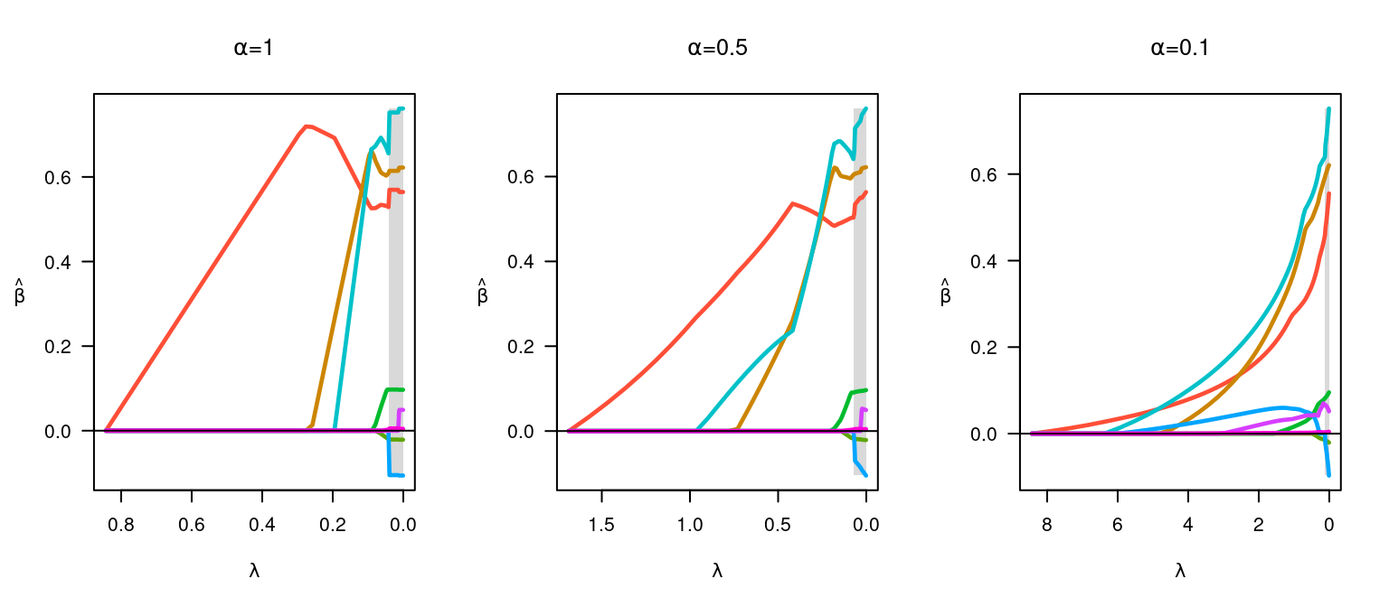
All of the above penalties can be combined with a ridge penalty. For example, we can add the lasso and ridge penalties (this is known as the elastic net):

P(\beta; \lambda, \alpha) = \alpha\lambda\left\lvert beta\right\rvert + (1 - \alpha) \lambda\beta^2

Here, alpha controls the tradeoff between the two penalties, with \alpha = 1 being identical to the lasso penalty and \alpha = 0 being identical to ridge. “MNet” (MCP + ridge) and “SCADNet” (SCAD + ridge) are formed similarly.

par(mfrow = c(1, 3))
fit <- ncvreg(x, y)
plot(fit, main = expression(paste(alpha, "=", 1)))
fit <- ncvreg(x, y, alpha = 0.5)
plot(fit, main = expression(paste(alpha, "=", 0.5)))
fit <- ncvreg(x, y, alpha = 0.1)
plot(fit, main = expression(paste(alpha, "=", 0.1)))

Patrick Breheny

MCP

SCAD

Lasso

Elastic Net and MNet