Model setting and notation
Let g = 1,\ldots,K index treatment groups and i = 1,\ldots,N_{\text{subj}} index subjects.
Subject i belongs to treatment group g_i \in \{1,\ldots,K\}.
Let V_{in} > 0 denote the observed tumor volume for subject i at time t_{in}, and define the log-volume
y_{in} = \log(V_{in}).
Model (log-volume scale)
Observation model (Level 1)
For each subject i and measurement n,
y_{in} \mid \alpha_i, \beta_i, \sigma \sim \mathcal{N}\left(\alpha_i + \beta_i t_{in}, \sigma^2\right),
where \alpha_i is the subject-specific intercept (baseline log-volume at t=0),
\beta_i is the subject-specific slope (log-scale growth rate),
and \sigma>0 is the residual standard deviation.
Subject-level random effects (Level 2)
Define the subject-specific parameter vector
\theta_i = \begin{pmatrix} \alpha_i \\ \beta_i \end{pmatrix}, \qquad \mu_g = \begin{pmatrix} \alpha_g \\ \beta_g \end{pmatrix}.
Conditional on the treatment group g_i,
\theta_i \mid g_i, \mu_{g_i}, \Sigma \sim \mathcal{N}_2(\mu_{g_i}, \Sigma).
We parameterize the random-effects covariance matrix as
\Sigma = D R D, \qquad D = \mathrm{diag}(\tau_\alpha,\tau_\beta), \qquad R = \begin{pmatrix} 1 & \rho \\ \rho & 1 \end{pmatrix},
where \tau_\alpha>0 and \tau_\beta>0 are the standard deviations of the random intercept and random slope, and \rho \in (-1,1) is their correlation.
Priors (Level 3)
For g=1,\ldots,K,
\alpha_g \sim \mathcal{N}(0,10^2), \qquad \beta_g \sim \mathcal{N}(0,10^2).
Residual standard deviation:
\sigma \sim \text{Half-}\mathcal{N}(0,5^2).
Random-effects standard deviations:
\tau_\alpha \sim \text{Half-}\mathcal{N}(0,5^2), \qquad \tau_\beta \sim \text{Half-}\mathcal{N}(0,5^2).
Correlation matrix prior:
R \sim \mathrm{LKJ}(2).
Summary
\begin{aligned} y_{in} \mid \alpha_i,\beta_i,\sigma &\sim \mathcal{N}(\alpha_i+\beta_i t_{in},\sigma^2),\\ \theta_i \mid g_i &\sim \mathcal{N}_2(\mu_{g_i}, \Sigma),\\ \alpha_g &\sim \mathcal{N}(0,10^2), \quad \beta_g \sim \mathcal{N}(0,10^2),\\ \sigma &\sim \text{Half-}\mathcal{N}(0,5^2),\\ \tau_\alpha,\tau_\beta &\sim \text{Half-}\mathcal{N}(0,5^2), \quad R \sim \mathrm{LKJ}(2). \end{aligned}
Example
Model fit
We begin by loading the example dataset and fitting the Bayesian hierarchical linear model using bhm(). By default, the model is estimated on the log scale.
Summary of the results
Posterior summaries can be obtained using the summary() method. The output reports posterior means and corresponding credible intervals for all estimated quantities, including:
Treatment-specific intercepts
Treatment-specific slopes
Pairwise treatment contrasts in slopes
summary(fit)$int_each
# A tibble: 5 × 7
treatment mean q5 q95 exp_mean exp_q5 exp_q95
<chr> <dbl> <dbl> <dbl> <dbl> <dbl> <dbl>
1 A 3.65 3.27 4.04 38.5 26.3 56.7
2 B 4.19 3.81 4.58 66.3 45.0 97.7
3 C 4.44 4.06 4.81 84.7 58.3 122.
4 D 4.99 4.61 5.37 147. 101. 216.
5 E 3.50 3.10 3.92 33.2 22.2 50.5
$slope_each
# A tibble: 5 × 10
treatment mean q5 q95 growth_factor_mean growth_factor_q5
<chr> <dbl> <dbl> <dbl> <dbl> <dbl>
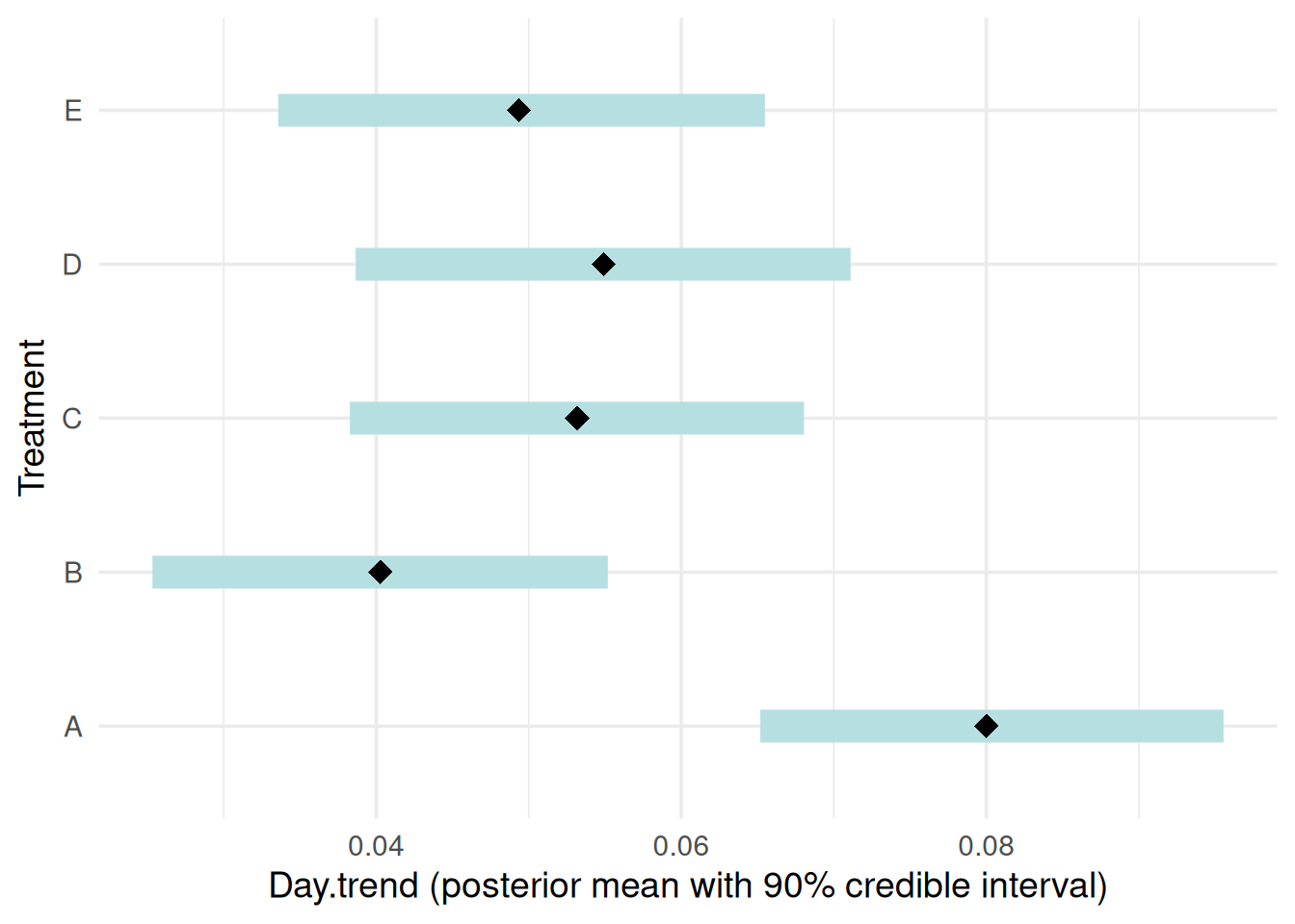
1 A 0.0800 0.0652 0.0956 1.08 1.07
2 B 0.0403 0.0253 0.0552 1.04 1.03
3 C 0.0532 0.0383 0.0680 1.05 1.04
4 D 0.0549 0.0386 0.0711 1.06 1.04
5 E 0.0494 0.0336 0.0655 1.05 1.03
# ℹ 4 more variables: growth_factor_q95 <dbl>, pct_change_mean <dbl>,
# pct_change_q5 <dbl>, pct_change_q95 <dbl>
$slope_diff
# A tibble: 10 × 10
contrast mean q5 q95 ratio_mean ratio_q5 ratio_q95
<chr> <dbl> <dbl> <dbl> <dbl> <dbl> <dbl>
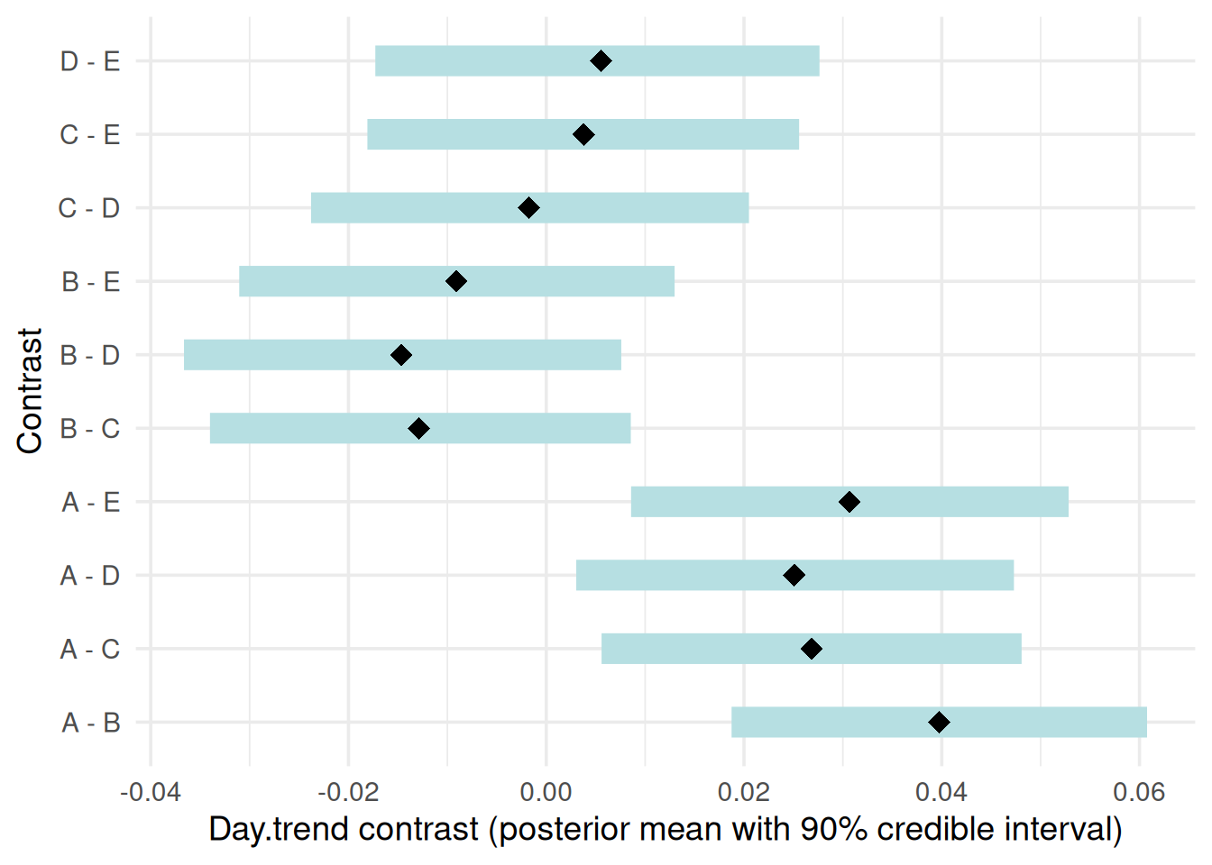
1 A - B 0.0397 0.0187 0.0608 1.04 1.02 1.06
2 A - C 0.0269 0.00559 0.0481 1.03 1.01 1.05
3 A - D 0.0251 0.00303 0.0473 1.03 1.00 1.05
4 A - E 0.0307 0.00858 0.0528 1.03 1.01 1.05
5 B - C -0.0129 -0.0340 0.00855 0.987 0.967 1.01
6 B - D -0.0147 -0.0366 0.00759 0.985 0.964 1.01
7 B - E -0.00909 -0.0311 0.0130 0.991 0.969 1.01
8 C - D -0.00176 -0.0238 0.0205 0.998 0.976 1.02
9 C - E 0.00380 -0.0181 0.0256 1.00 0.982 1.03
10 D - E 0.00556 -0.0173 0.0276 1.01 0.983 1.03
# ℹ 3 more variables: pct_diff_mean <dbl>, pct_diff_q5 <dbl>,
# pct_diff_q95 <dbl>Plots
Posterior results can be visualized using the plot() method with different type options. The available plot types include:
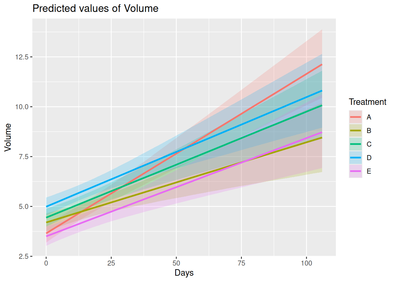
“predict”: Posterior predicted treatment-specific mean trajectories
“slope”: Posterior summaries of treatment-specific slopes with 90% credible intervals
“contrast”: Pairwise contrasts in slopes between treatment groups with 90% credible intervals
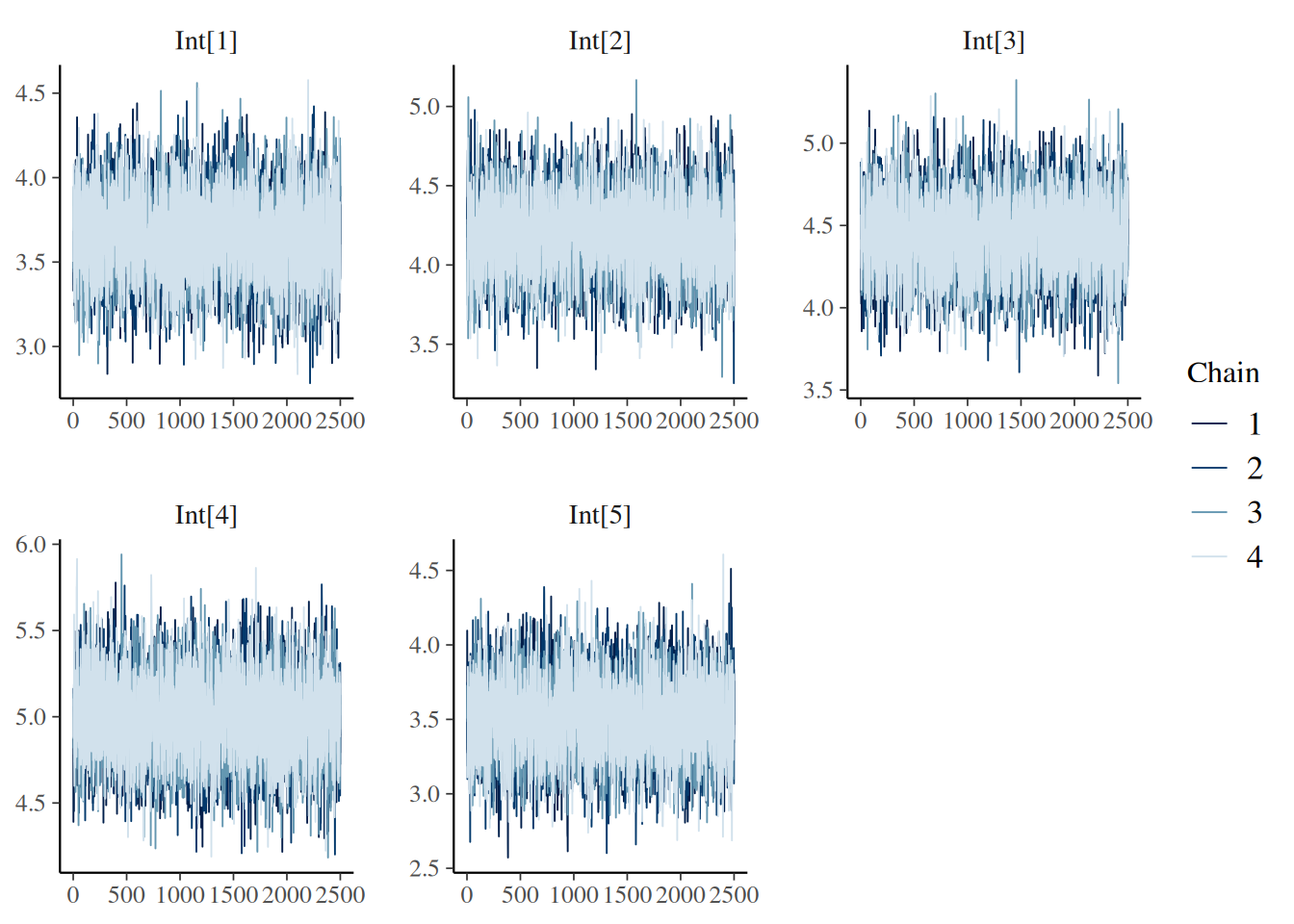
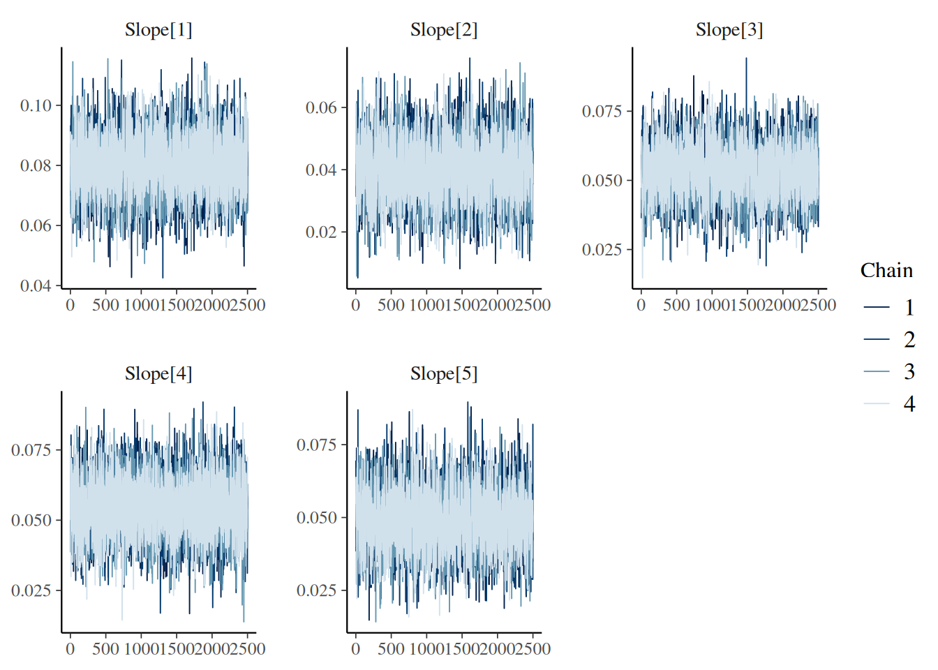
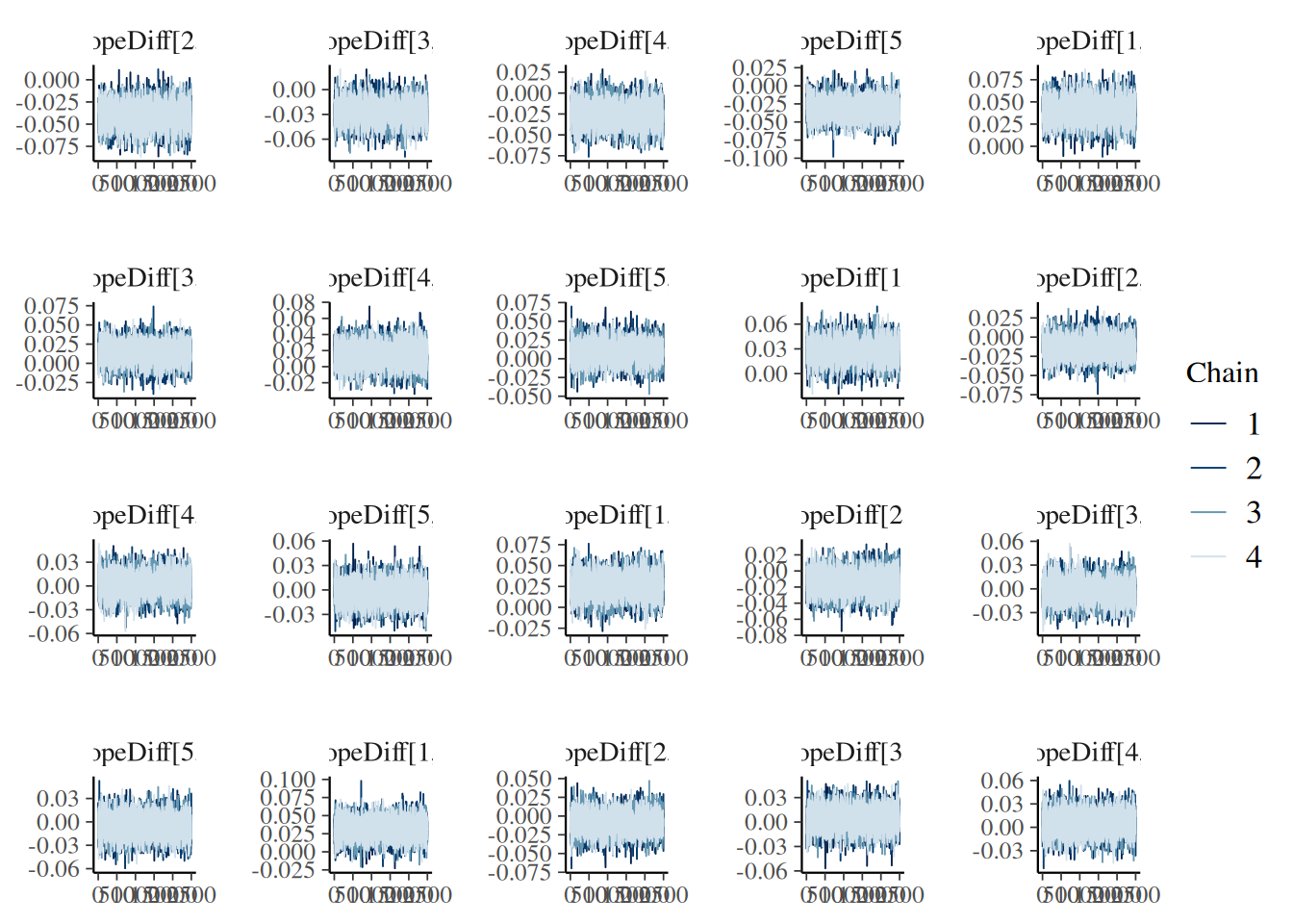
“trace”: MCMC trace plots for model diagnostics