Convergence Failure with lmm()
If you encounter the warning
“Model failed to converge with max|grad|”
when fitting a model with lmm(), one common cause is poor scaling of the time variable. A simple and effective fix is to rescale time to a larger unit (for example, from days to months).
Example
Using the melanoma2 dataset, the following code produces a convergence warning:
data(melanoma2)
mel2 <- tumr(melanoma2, ID, Day, Volume, Treatment)
lmm(mel2)
Warning in checkConv(attr(opt, "derivs"), opt$par, ctrl = control$checkConv, : Model failed to converge with max|grad| = 0.00566844 (tol = 0.002, component 1)
  See ?lme4::convergence and ?lme4::troubleshooting.
Linear mixed model fit by REML. t-tests use Satterthwaite's method [
lmerModLmerTest]
Formula: log1p(Volume) ~ Treatment * Day + (Day | ID)
   Data: data

REML criterion at convergence: 1216.5

Scaled residuals:
    Min      1Q  Median      3Q     Max
-6.8683 -0.3590  0.0569  0.4891  4.0759

Random effects:
 Groups   Name        Variance  Std.Dev. Corr
 ID       (Intercept) 0.3909753 0.62528
          Day         0.0006511 0.02552  -0.51
 Residual             0.3220706 0.56751
Number of obs: 568, groups:  ID, 47

Fixed effects:
               Estimate Std. Error       df t value Pr(>|t|)
(Intercept)     3.66092    0.22688 46.83127  16.136  < 2e-16 ***
TreatmentB      0.53834    0.32255 42.89746   1.669  0.10240
TreatmentC      0.78053    0.31957 46.08359   2.442  0.01848 *
TreatmentD      1.33290    0.32410 48.71755   4.113  0.00015 ***
TreatmentE     -0.14693    0.33197 42.42209  -0.443  0.66031
Day             0.07971    0.00897 47.89633   8.886 1.06e-11 ***
TreatmentB:Day -0.03972    0.01269 43.36203  -3.130  0.00312 **
TreatmentC:Day -0.02673    0.01255 46.24553  -2.129  0.03859 *
TreatmentD:Day -0.02497    0.01321 54.20921  -1.890  0.06410 .
TreatmentE:Day -0.03060    0.01300 42.19464  -2.355  0.02325 *
---
Signif. codes:  0 '***' 0.001 '**' 0.01 '*' 0.05 '.' 0.1 ' ' 1

Correlation of Fixed Effects:
            (Intr) TrtmnB TrtmnC TrtmnD TrtmnE Day    TrtB:D TrtC:D TrtD:D
TreatmentB  -0.703
TreatmentC  -0.710  0.499
TreatmentD  -0.700  0.492  0.497
TreatmentE  -0.683  0.481  0.485  0.478
Day         -0.577  0.406  0.410  0.404  0.394
TretmntB:Dy  0.408 -0.560 -0.290 -0.286 -0.279 -0.707
TretmntC:Dy  0.412 -0.290 -0.573 -0.289 -0.282 -0.715  0.505
TretmntD:Dy  0.392 -0.276 -0.278 -0.585 -0.268 -0.679  0.480  0.485
TretmntE:Dy  0.398 -0.280 -0.283 -0.279 -0.556 -0.690  0.488  0.493  0.469
optimizer (nloptwrap) convergence code: 0 (OK)
Model failed to converge with max|grad| = 0.00566844 (tol = 0.002, component 1)
  See ?lme4::convergence and ?lme4::troubleshooting.
Solution: Rescale the Time Variable
In this case, converting time from days to months resolves the convergence issue. Below, we create a new time variable by dividing by the average number of days per month, update the tumr object, and refit the model:
melanoma2$months <- melanoma2$Day / (365/12)
mel2 <- tumr(melanoma2, ID, months, Volume, Treatment)
lmm(mel2)
Linear mixed model fit by REML. t-tests use Satterthwaite's method [
lmerModLmerTest]
Formula: log1p(Volume) ~ Treatment * months + (months | ID)
   Data: data

REML criterion at convergence: 1182.4

Scaled residuals:
    Min      1Q  Median      3Q     Max
-6.8683 -0.3590  0.0569  0.4891  4.0759

Random effects:
 Groups   Name        Variance Std.Dev. Corr
 ID       (Intercept) 0.3911   0.6254
          months      0.6025   0.7762   -0.51
 Residual             0.3221   0.5675
Number of obs: 568, groups:  ID, 47

Fixed effects:
                  Estimate Std. Error      df t value Pr(>|t|)
(Intercept)         3.6609     0.2269 46.8170  16.134  < 2e-16 ***
TreatmentB          0.5383     0.3226 42.8852   1.669  0.10244
TreatmentC          0.7805     0.3196 46.0697   2.442  0.01849 *
TreatmentD          1.3329     0.3241 48.7024   4.112  0.00015 ***
TreatmentE         -0.1469     0.3320 42.4100  -0.443  0.66031
months              2.4245     0.2729 47.8797   8.885 1.07e-11 ***
TreatmentB:months  -1.2083     0.3860 43.3477  -3.130  0.00312 **
TreatmentC:months  -0.8130     0.3818 46.2297  -2.129  0.03861 *
TreatmentD:months  -0.7594     0.4018 54.1899  -1.890  0.06412 .
TreatmentE:months  -0.9309     0.3953 42.1808  -2.355  0.02327 *
---
Signif. codes:  0 '***' 0.001 '**' 0.01 '*' 0.05 '.' 0.1 ' ' 1

Correlation of Fixed Effects:
            (Intr) TrtmnB TrtmnC TrtmnD TrtmnE months TrtmB: TrtmC: TrtmD:
TreatmentB  -0.703
TreatmentC  -0.710  0.499
TreatmentD  -0.700  0.492  0.497
TreatmentE  -0.683  0.481  0.485  0.478
months      -0.577  0.406  0.410  0.404  0.395
TrtmntB:mnt  0.408 -0.560 -0.290 -0.286 -0.279 -0.707
TrtmntC:mnt  0.413 -0.290 -0.573 -0.289 -0.282 -0.715  0.505
TrtmntD:mnt  0.392 -0.276 -0.278 -0.586 -0.268 -0.679  0.480  0.485
TrtmntE:mnt  0.398 -0.280 -0.283 -0.279 -0.556 -0.690  0.488  0.493  0.469
After rescaling the time variable, the model fits without producing the convergence warning.
Why This Works
Rescaling time can improve numerical stability during optimization, making it easier for the model to converge—especially when time values are large or measured on a very fine scale.
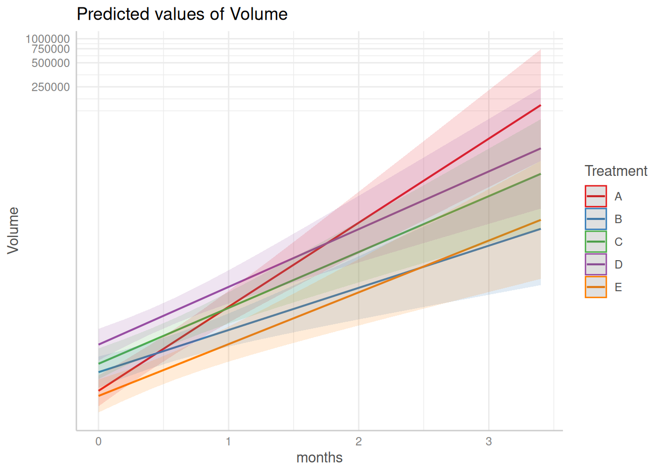
Putting lmm() Summary Plot on the Log Scale
When viewing the summary plot from lmm(), you may see the message:
“Model has log1p-transformed response. Back-transforming predictions to original response scale.Standard errors are still on the transformed scale.”
This message appears because lmm() fits the model using a log1p-transformed response by default, and the plot() method automatically back-transforms predicted values to the original response scale.
If you prefer to view the predicted volume values on the log scale, you can apply a log transformation directly to the plot’s y-axis. Since the summary plot is a ggplot2 object, this can be done using scale_y_continuous() with a log1p transformation from the scales package.
Model has log1p-transformed response. Back-transforming predictions to
  original response scale. Standard errors are still on the transformed
  scale.
Scale for y is already present.
Adding another scale for y, which will replace the existing scale.
This approach preserves the model fit while allowing you to visualize predictions and uncertainty on the transformed scale.
The lmm() function allows you to override the default model formula, providing flexibility when fitting alternative model specifications.
By default, lmm() fits a model of the form log1p(measure) ~ group * time + (time | id) (for example, Volume ~ months + (1 | ID)).
In the example below, the default formula is replaced with a simpler model that uses a rescaled time variable and a random intercept only:
lmm_mel2 <- lmm(
                 tumr_obj = mel2,
                 formula = "Volume ~ months + (1 | ID)"
               )
While the model fits successfully, calling summary() on this object will fail.
This occurs because the summary() method is designed around the default lmm() model structure and currently assumes that formula. As a result, alternative formulas may not be fully supported by summary().
When using a custom formula, keep in mind that some downstream methods—such as summary()—may not behave as expected.