Getting started with ncvreg

ncvreg is an R package for fitting regularization paths for linear regression, GLM, and Cox regression models using lasso or nonconvex penalties, in particular the minimax concave penalty (MCP) and smoothly clipped absolute deviation (SCAD) penalty, with options for additional L₂ penalties (the “elastic net” idea). Utilities for carrying out cross-validation as well as post-fitting visualization, summarization, inference, and prediction are also provided.

ncvreg comes with a few example data sets; we’ll look at Prostate, which has 8 features and one continuous response, the PSA levels (on the log scale) from men about to undergo radical prostatectomy:

data(Prostate)
X <- Prostate$X
y <- Prostate$y

To fit a penalized regression model to this data:

fit <- ncvreg(X, y)

The default penalty here is the minimax concave penalty (MCP), but SCAD and lasso penalties are also available. This produces a path of coefficients, which we can plot with

plot(fit)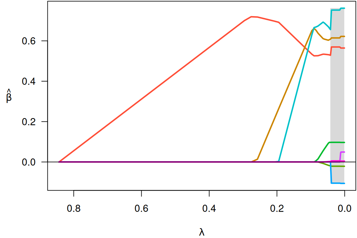

Notice that variables enter the model one at a time, and that at any given value of \lambda, several coefficients are zero. To see what the coefficients are, we could use the coef function:

coef(fit, lambda=0.05)
# (Intercept)      lcavol     lweight         age        lbph         svi 
#  0.35121089  0.53178994  0.60389694 -0.01530917  0.08874563  0.67256096 
#         lcp     gleason       pgg45 
#  0.00000000  0.00000000  0.00168038

The summary method can be used for post-selection inference:

summary(fit, lambda=0.05)
# MCP-penalized linear regression with n=97, p=8
# At lambda=0.0500:
# -------------------------------------------------
#   Nonzero coefficients         :   6
#   Expected nonzero coefficients:   2.54
#   Average mfdr (6 features)    :   0.424
# 
#         Estimate      z     mfdr Selected
# lcavol   0.53179  8.880  < 1e-04        *
# svi      0.67256  3.945 0.010189        *
# lweight  0.60390  3.666 0.027894        *
# lbph     0.08875  1.928 0.773014        *
# age     -0.01531 -1.788 0.815269        *
# pgg45    0.00168  1.160 0.917570        *

In this case, it would appear that lcavol, svi, and lweight are clearly associated with the response, even after adjusting for the other variables in the model, while lbph, age, and pgg45 may be false positives included simply by chance.

Typically, one would carry out cross-validation for the purposes of assessing the predictive accuracy of the model at various values of \lambda:

cvfit <- cv.ncvreg(X, y)
summary(cvfit)
# MCP-penalized linear regression with n=97, p=8
# At minimum cross-validation error (lambda=0.0169):
# -------------------------------------------------
#   Nonzero coefficients: 7
#   Cross-validation error (deviance): 0.55
#   R-squared: 0.59
#   Signal-to-noise ratio: 1.42
#   Scale estimate (sigma): 0.739
plot(cvfit)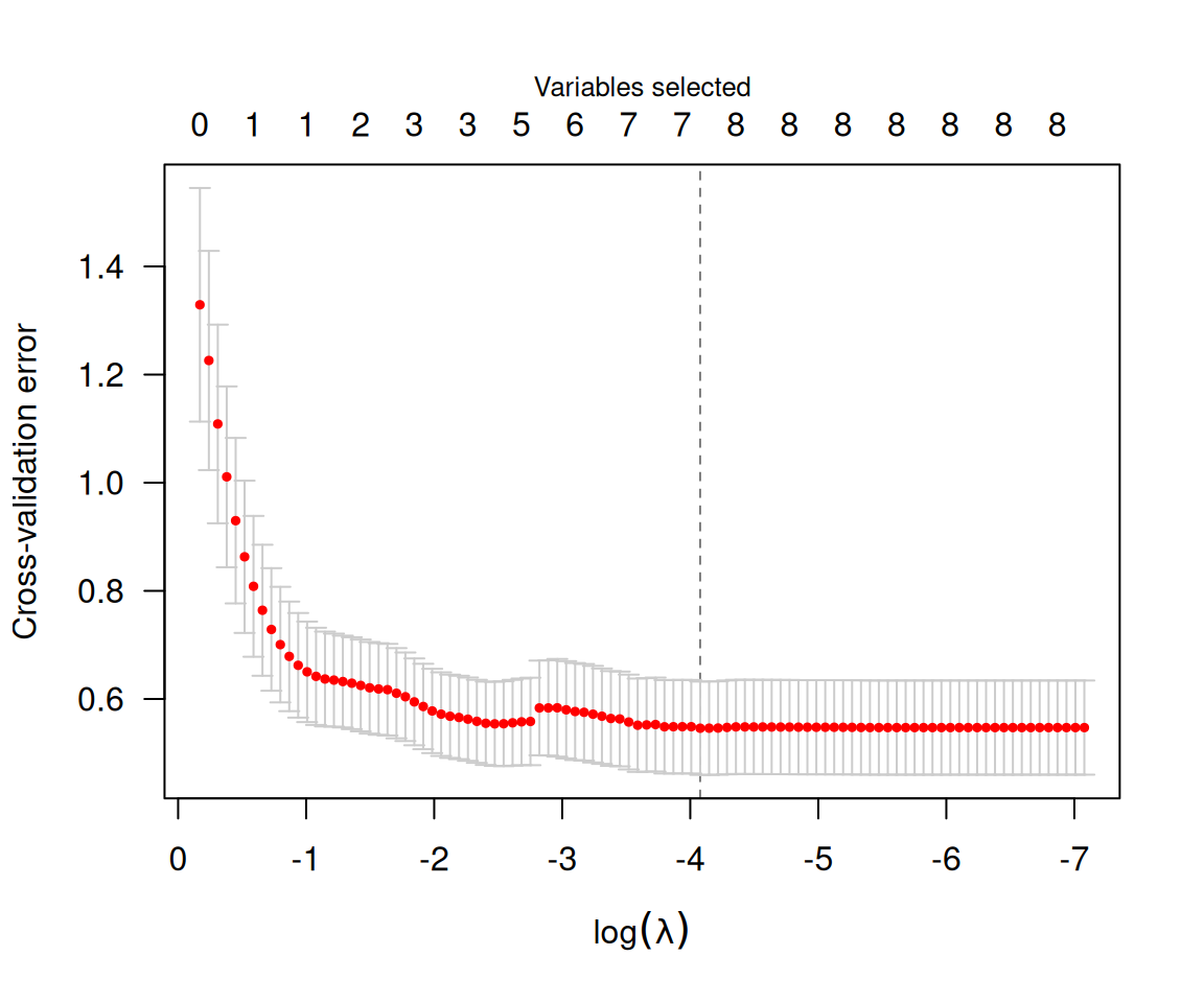

The value of \lambda that minimizes the cross-validation error is given by cvfit$lambda.min, which in this case is 0.017. Applying coef to the output of cv.ncvreg returns the coefficients at that value of \lambda:

coef(cvfit)
#  (Intercept)       lcavol      lweight          age         lbph          svi 
#  0.494154801  0.569546027  0.614419811 -0.020913467  0.097352536  0.752397339 
#          lcp      gleason        pgg45 
# -0.104959403  0.000000000  0.005324465

Predicted values can be obtained via predict, which has a number of options:

predict(cvfit, X=head(X))     # Prediction of response for new observations
#         1         2         3         4         5         6 
# 0.8304040 0.7650906 0.4262072 0.6230117 1.7449492 0.8449595
predict(cvfit, type="nvars")  # Number of nonzero coefficients
# 0.01695 
#       7
predict(cvfit, type="vars")   # Identity of the nonzero coefficients
#  lcavol lweight     age    lbph     svi     lcp   pgg45 
#       1       2       3       4       5       6       8

Note that the original fit (to the full data set) is returned as cvfit$fit; it is not necessary to call both ncvreg and cv.ncvreg to analyze a data set. For example, plot(cvfit$fit) will produce the same coefficient path plot as plot(fit) above.

Patrick Breheny