Fit a linear mixed model via non-convex penalized maximum likelihood.

Usage

plmm(
  design,
  K = NULL,
  diag_K = NULL,
  eta_star = NULL,
  penalty = "lasso",
  init = NULL,
  gamma,
  alpha = 1,
  dfmax = NULL,
  lambda_min,
  nlambda = 100,
  lambda,
  eps = 1e-04,
  max_iter = 10000,
  convex = TRUE,
  warn = TRUE,
  trace = FALSE,
  save_rds = NULL,
  compact_save = FALSE,
  return_fit = NULL,
  ...
)

Arguments

design: A plmm_design object (as created by create_design()) or a string with the file path to a design object (the file path must end in '.rds').
K: Similarity matrix used to rotate the data. This should either be: (1) a known matrix that reflects the covariance of y, (2) an estimate (Default is \(\frac{1}{p}(XX^T)\)), or (3) a list with components 'd' and 'U', as returned by a previous plmm() model fit on the same data.
diag_K: Logical: should K be a diagonal matrix? This would reflect observations that are unrelated, or that can be treated as unrelated. Defaults to FALSE. Note: plmm() does not check to see if a matrix is diagonal. If you want to use a diagonal K matrix, you must set diag_K = TRUE.
eta_star: Optional argument to input a specific eta term rather than estimate it from the data. If K is a known covariance matrix that is full rank, this should be 1.
penalty: The penalty to be applied to the model. Either "lasso" (the default), "SCAD", or "MCP".
init: Initial values for coefficients. Default is 0 for all columns of X.
gamma: The tuning parameter of the MCP/SCAD penalty (see details). Default is 3 for MCP and 3.7 for SCAD.
alpha: Tuning parameter for the Mnet estimator which controls the relative contributions from the MCP/SCAD penalty and the ridge, or L2 penalty. alpha=1 is equivalent to MCP/SCAD penalty, while alpha=0 would be equivalent to ridge regression. However, alpha=0 is not supported; alpha may be arbitrarily small, but not exactly 0.
dfmax: (Future idea; not yet incorporated): Upper bound for the number of nonzero coefficients. Default is no upper bound. However, for large data sets, computational burden may be heavy for models with a large number of nonzero coefficients.
lambda_min: The smallest value for lambda, as a fraction of lambda.max. Default is .001 if the number of observations is larger than the number of covariates and .05 otherwise.
nlambda: Length of the sequence of lambda. Default is 100.
lambda: A user-specified sequence of lambda values. By default, a sequence of values of length nlambda is computed, equally spaced on the log scale.
eps: Convergence threshold. The algorithm iterates until the RMSD for the change in linear predictors for each coefficient is less than eps. Default is 1e-4.
max_iter: Maximum number of iterations (total across entire path). Default is 10000.
convex: (Future idea; not yet incorporated): Calculate index for which objective function ceases to be locally convex? Default is TRUE.
warn: Return warning messages for failures to converge and model saturation? Default is TRUE.
trace: If set to TRUE, inform the user of progress by announcing the beginning of each step of the modeling process. Default is FALSE.
save_rds: Optional: if a filepath and name without the '.rds' suffix is specified (e.g., save_rds = "~/dir/my_results"), then the model results are saved to the provided location (e.g., "~/dir/my_results.rds"). Defaults to NULL, which does not save the result.
compact_save: Optional: if TRUE, three separate .rds files will saved: one with the 'beta_vals', one with 'K', and one with everything else (see below). Defaults to FALSE. Note: you must specify save_rds for this argument to be called.
return_fit: Optional: a logical value indicating whether the fitted model should be returned as a plmm object in the current (assumed interactive) session. Defaults to TRUE for in-memory data, and defaults to FALSE for filebacked data.
...: Additional optional arguments to plmm_checks()

Value

A list which includes:

beta_vals: the matrix of estimated coefficients on the original scale. Rows are predictors, columns are values of lambda
rotated_scale_beta_vals: the matrix of estimated coefficients on the ~rotated~ scale. This is the scale on which the model was fit.
lambda: a numeric vector of the lasso tuning parameter values used in model fitting.
eta: a number (double) between 0 and 1 representing the estimated proportion of the variance in the outcome attributable to population/correlation structure
linear_predictors: the matrix resulting from the product of stdrot_X and the estimated coefficients on the ~rotated~ scale.
penalty: character string indicating the penalty with which the model was fit (e.g., 'MCP')
gamma: numeric value indicating the tuning parameter used for the SCAD or lasso penalties was used. Not relevant for lasso models.
alpha: numeric value indicating the elastic net tuning parameter.
loss: vector with the numeric values of the loss at each value of lambda (calculated on the ~rotated~ scale)
penalty_factor: vector of indicators corresponding to each predictor, where 1 = predictor was penalized.
ns_idx: vector with the indices of predictors which were non-singular features (i.e., features which had variation).
iter: numeric vector with the number of iterations needed in model fitting for each value of lambda
converged: vector of logical values indicating whether the model fitting converged at each value of lambda
K: a list with 2 elements, s and U —
- s: a vector of the eigenvalues of the relatedness matrix; see relatedness_mat() for details.
- U: a matrix of the eigenvectors of the relatedness matrix

Examples

# using admix data
admix_design <- create_design(X = admix$X, outcome_col = admix$y)
fit_admix1 <- plmm(design = admix_design)
s1 <- summary(fit_admix1, idx = 50)
print(s1)
#> lasso-penalized regression model with n=197, p=101 at lambda=0.01380
#> -------------------------------------------------
#> The model converged 
#> -------------------------------------------------
#> # of non-zero coefficients:  85 
#> -------------------------------------------------
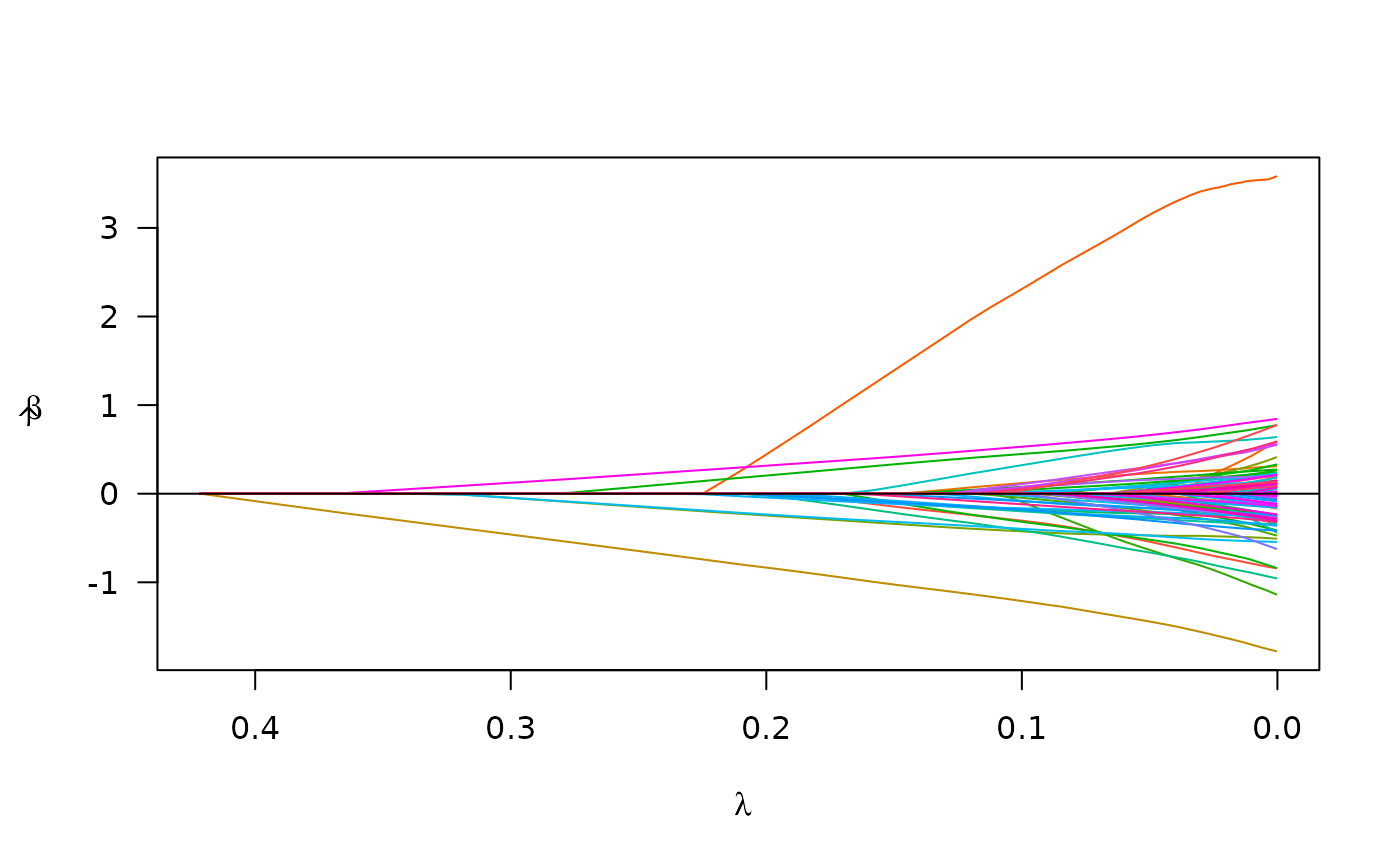
plot(fit_admix1)


# Note: for examples with large data that are too big to fit in memory,
# see the article "PLINK files/file-backed matrices" on our website
# https://pbreheny.github.io/plmmr/articles/filebacking.html