If your data is in a matrix or data frame

library(plmmr)
#> Loading required package: bigalgebra
#> Loading required package: bigmemory

In this overview, I will provide a demo of the main functions in plmmr using the admix data. Checkout the other vignettes to see examples of analyzing data from PLINK files or delimited files.

Examine what we have in the admix data:

str(admix)
#> List of 3
#>  $ X   : int [1:197, 1:100] 0 0 0 0 1 0 1 0 0 0 ...
#>   ..- attr(*, "dimnames")=List of 2
#>   .. ..$ : NULL
#>   .. ..$ : chr [1:100] "Snp1" "Snp2" "Snp3" "Snp4" ...
#>  $ y   : num [1:197, 1] 3.52 3.754 1.191 0.579 4.085 ...
#>  $ race: num [1:197] 1 1 1 1 1 1 1 1 1 1 ...

Preparing data for analysis

The first step with in-memory data is creating a plmm_design object, which we do with create_design() like this:

admix_design <- create_design(X = admix$X, outcome_col = admix$y)
str(admix_design)
#> List of 12
#>  $ std_X         : num [1:197, 1:98] -0.398 -0.398 -0.398 -0.398 2.053 ...
#>   ..- attr(*, "dimnames")=List of 2
#>   .. ..$ : NULL
#>   .. ..$ : chr [1:98] "Snp1" "Snp2" "Snp3" "Snp4" ...
#>   ..- attr(*, "center")= num [1:100] 0.16244 0.15228 0.00508 0.30964 0.01015 ...
#>   ..- attr(*, "scale")= num [1:100] 0.4081 0.3593 0.0711 0.5793 0.1002 ...
#>   ..- attr(*, "nonsingular")= int [1:98] 1 2 3 4 5 6 7 9 10 11 ...
#>  $ std_X_n       : int 197
#>  $ std_X_p       : int 98
#>  $ ns            : int [1:98] 1 2 3 4 5 6 7 9 10 11 ...
#>  $ std_X_center  : num [1:100] 0.16244 0.15228 0.00508 0.30964 0.01015 ...
#>  $ std_X_scale   : num [1:100] 0.4081 0.3593 0.0711 0.5793 0.1002 ...
#>  $ X_colnames    : chr [1:100] "Snp1" "Snp2" "Snp3" "Snp4" ...
#>  $ n             : int 197
#>  $ p             : int 100
#>  $ y             : num [1:197, 1] 3.52 3.754 1.191 0.579 4.085 ...
#>  $ std_X_colnames: chr [1:98] "Snp1" "Snp2" "Snp3" "Snp4" ...
#>  $ penalty_factor: num [1:98] 1 1 1 1 1 1 1 1 1 1 ...
#>  - attr(*, "class")= chr "plmm_design"

‘Creating a design’ means that we take the processed data and create the three essential elements for data analysis: a design matrix that is column-standardized, an outcome vector, and a penalty factor indicator. In our math notation, the design matrix is \mathbf{X}, the outcome vector is \mathbf{y}, and the penalty factor indicator is a vector of 1s and 0s, where 1s correspond to the features in \mathbf{X} that will be penalized (and the 0s correspond to the unpenalized added predictors). Note that in our current admix_design, all features are penalized (i.e., the penalty factor is a vector of 1).

Basic model fitting

The admix dataset is now ready to analyze with a call to plmmr::plmm() (one of the main functions in plmmr):

admix_fit <- plmm(design = admix_design)
summary(admix_fit, lambda = admix_fit$lambda[50])
#> lasso-penalized regression model with n=197, p=101 at lambda=0.01380
#> -------------------------------------------------
#> The model converged 
#> -------------------------------------------------
#> # of non-zero coefficients:  85 
#> -------------------------------------------------

The returned beta_vals item is a matrix whose rows are \hat\beta coefficients and whose columns represent values of the penalization parameter \lambda. By default, plmm fits 100 values of \lambda (see the setup_lambda function for details).

admix_fit$beta_vals[1:10, 97:100] |> 
  knitr::kable(digits = 3,
               format = "html")

	0.00052	0.00048	0.00045	0.00042
(Intercept)	7.020	7.021	7.022	7.022
Snp1	-0.841	-0.841	-0.841	-0.842
Snp2	0.199	0.199	0.199	0.199
Snp3	3.580	3.581	3.581	3.581
Snp4	0.189	0.190	0.190	0.190
Snp5	0.588	0.588	0.589	0.589
Snp6	-0.135	-0.135	-0.135	-0.135
Snp7	0.207	0.208	0.208	0.208
Snp8	0.000	0.000	0.000	0.000
Snp9	0.310	0.310	0.310	0.310

Note that for all values of \lambda, SNP 8 has \hat \beta = 0. This is because SNP 8 is a constant feature, a feature (i.e., a column of \mathbf{X}) whose values do not vary among the members of this population.

We can summarize our fit at the nth \lambda value:

# for n = 25 
summary(admix_fit, lambda = admix_fit$lambda[25])
#> lasso-penalized regression model with n=197, p=101 at lambda=0.07896
#> -------------------------------------------------
#> The model converged 
#> -------------------------------------------------
#> # of non-zero coefficients:  46 
#> -------------------------------------------------

We can also plot the path of the fit to see how model coefficients vary with \lambda:

plot(admix_fit)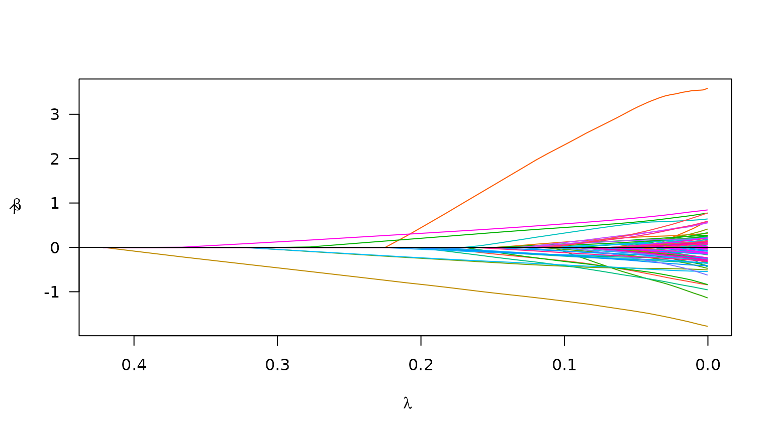

Plot of path for model fit

Suppose we also know the ancestry groups with which for each person in the admix data self-identified. We would probably want to include this in the model as an unpenalized covariate (i.e., we would want ‘ancestry’ to always be in the model). Here is how that could look:

X_plus_ancestry <- cbind(admix$race, admix$X)
colnames(X_plus_ancestry) <- c("ancestry", colnames(admix$X))

# create a new design
admix_design2 <- create_design(X = X_plus_ancestry,
                               outcome_col = admix$y,
                               # below, I mark ancestry variable as unpenalized
                               # we want ancestry to always be in the model
                               unpen = "ancestry")

# now fit a model 
admix_fit2 <- plmm(design = admix_design2, 
                   outcome_col = admix$y)

We may compare the results from the model which includes ‘ancestry’ to our first model:

summary(admix_fit2, idx = 25)
#> lasso-penalized regression model with n=197, p=102 at lambda=0.09986
#> -------------------------------------------------
#> The model converged 
#> -------------------------------------------------
#> # of non-zero coefficients:  15 
#> -------------------------------------------------
plot(admix_fit2)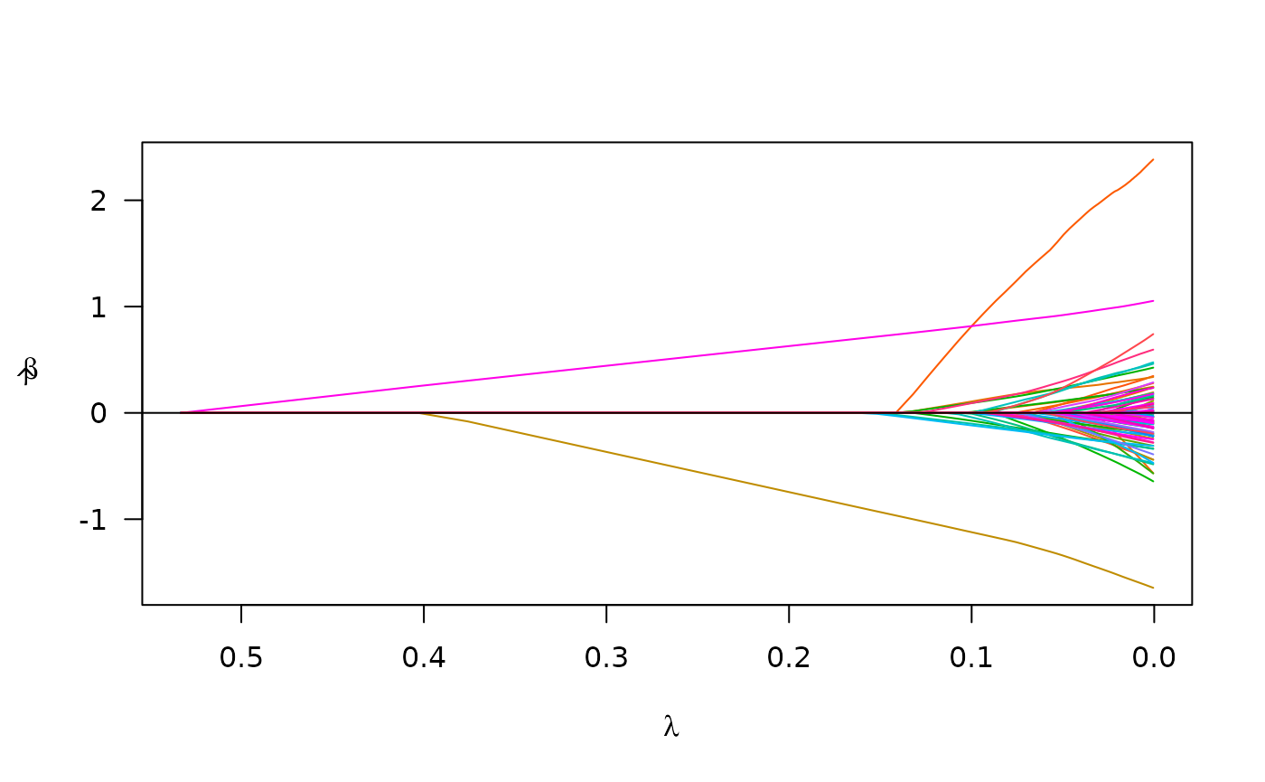

Cross validation

To select a \lambda value, we often use cross validation. Below is an example of using cv_plmm to select a \lambda that minimizes cross-validation error:

admix_cv <- cv_plmm(design = admix_design2, return_fit = T)

admix_cv_s <- summary(admix_cv, lambda = "min")
print(admix_cv_s)
#> lasso-penalized model with n=197 and p=102
#> At minimum cross-validation error (lambda=0.1871):
#> -------------------------------------------------
#>   Nonzero coefficients: 3
#>   Cross-validation error (deviance): 1.31
#>   Scale estimate (sigma): 1.145

We can also plot the cross-validation error (CVE) versus \lambda (on the log scale):

plot(admix_cv)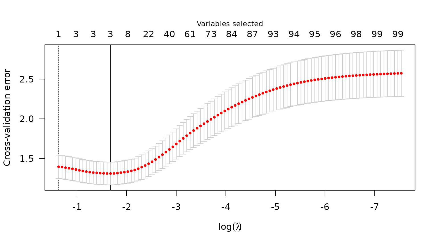

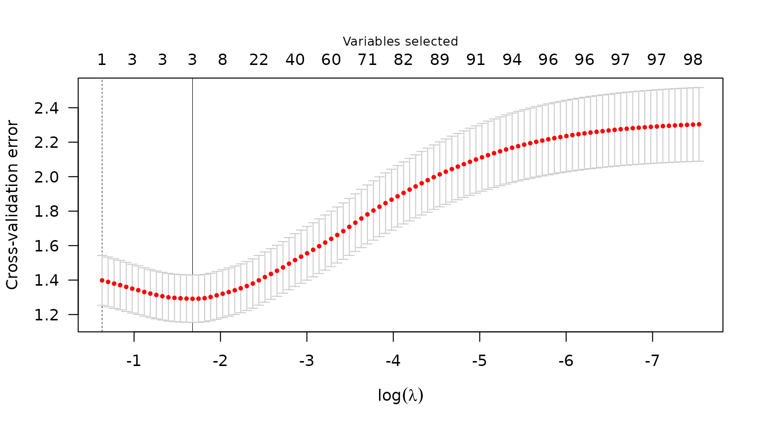
Plot of CVE

Predicted values

Below is an example of the predict() methods for PLMMs:

# make predictions for select lambda value(s)
y_hat <- predict(object = admix_fit,
                       newX = admix$X,
                       type = "blup",
                       X = admix$X,
                       y = admix$y)

We can compare these predictions with the predictions we would get from an intercept-only model using mean squared prediction error (MSPE) – lower is better:

# intercept-only (or 'null') model
crossprod(admix$y - mean(admix$y))/length(admix$y)
#>          [,1]
#> [1,] 5.928528

# our model at its best value of lambda
apply(y_hat, 2, function(c){crossprod(admix$y - c)/length(c)}) -> mse
min(mse)
#> [1] 0.9259769
# ^ across all values of lambda, our model has MSPE lower than the null model

We see our model has better predictions than the null.