A widely-used format for storing data from genome-wide association
studies (GWAS) is the PLINK file
formats, which consists of a triplet of .bed,
.bed, and .fam files. The plmmr
package is equipped to analyze data from PLINK files. If you have data
in this format, keep reading – if you want to know more about what each
of these files contains, see this
other tutorial or the PLINK documentation.
If your data is in delimited files (e.g., .txt,
.csv, etc.), read the article on analyzing data from
delimited files at
vignette("delim_files", package = "plmmr").
The plmmr package is designed to handle data so that
users can analyze large data sets. For this reason, data must be
preprocessed into a specific format. There are two steps to prepare for
analysis: (1) process the data and (2) create a design. Processing the
data means that we take the feature data and create a .rds
object that contains your feature data in a format compatible with the
bigmemory package.
Creating a design involves standardizing the input of the features,
outcome, and penalty factor for use in the modeling functions
plmm() and cv_plmm().
Processing PLINK files
First, unzip your PLINK files if they are zipped. Our example
penncath_lite data that ships with plmmr is
zipped; you can run this command to unzip:
temp_dir <- tempdir() # using a temp dir -- change to fit your preference
unzip_example_data(outdir = temp_dir)
#> Unzipped files are saved in /tmp/RtmpS9WXLH
For GWAS data, we have to tell plmmr how to combine
information across all three PLINK files (the .bed,
.bim, and .fam files). We do this with
process_plink().
Here, we will create the files we want in a temporary directory for
the sake of example. Users can specify the folder of their choice for
rds_dir, as shown below:
# temp_dir <- tempdir() # using a temporary directory (if you didn't already create one above)
plink_data <- process_plink(data_dir = temp_dir,
                            data_prefix = "penncath_lite",
                            rds_dir = temp_dir,
                            rds_prefix = "imputed_penncath_lite",
                            # imputing the mode to address missing values
                            impute_method = "mode",
                            # overwrite existing files in temp_dir
                            # (you can turn this feature off if you need to)
                            overwrite = TRUE,
                            # turning off parallelization -
                            #   leaving this on causes problems knitting this vignette
                            parallel = FALSE)
#> Preprocessing penncath_lite data...
#> Creating penncath_lite.rds
#> There are 1401 observations and 4367 genomic features in the specified data files, representing chromosomes 1 - 22 .
#> There are a total of 3514 SNPs with missing values.
#> Of these, 13 are missing in at least 50% of the samples.
#> Done with imputation.
#> process_plink() completed.
#> Processed files now saved as /tmp/RtmpS9WXLH/imputed_penncath_lite.rds
You’ll see a lot of messages printed to the console here … the result
of all this is the creation of 3 files:
imputed_penncath_lite.rds and
imputed_penncath_lite.bk contain the data. 1 These will show up in
the folder where the PLINK data is. What is returned is a filepath. The
.rds object at this filepath contains the processed data,
which we will now use to create our design.
For didactic purposes, let’s examine what’s in
imputed_penncath_lite.rds using the readRDS()
function (Note: Don’t do this in your analysis - the
section below reads the data into memory. This is just for
illustration):
pen <- readRDS(plink_data) # notice: this is a `processed_plink` object
str(pen) # note: genotype data is *not* in memory
#> List of 5
#>  $ X  :Formal class 'big.matrix.descriptor' [package "bigmemory"] with 1 slot
#>   .. ..@ description:List of 13
#>   .. .. ..$ sharedType: chr "FileBacked"
#>   .. .. ..$ filename  : chr "imputed_penncath_lite.bk"
#>   .. .. ..$ dirname   : chr "/tmp/RtmpS9WXLH/"
#>   .. .. ..$ totalRows : int 1401
#>   .. .. ..$ totalCols : int 4367
#>   .. .. ..$ rowOffset : num [1:2] 0 1401
#>   .. .. ..$ colOffset : num [1:2] 0 4367
#>   .. .. ..$ nrow      : num 1401
#>   .. .. ..$ ncol      : num 4367
#>   .. .. ..$ rowNames  : NULL
#>   .. .. ..$ colNames  : NULL
#>   .. .. ..$ type      : chr "double"
#>   .. .. ..$ separated : logi FALSE
#>  $ map:'data.frame': 4367 obs. of  6 variables:
#>   ..$ chromosome  : int [1:4367] 1 1 1 1 1 1 1 1 1 1 ...
#>   ..$ marker.ID   : chr [1:4367] "rs3107153" "rs2455124" "rs10915476" "rs4592237" ...
#>   ..$ genetic.dist: int [1:4367] 0 0 0 0 0 0 0 0 0 0 ...
#>   ..$ physical.pos: int [1:4367] 2056735 3188505 4275291 4280630 4286036 4302161 4364564 4388885 4606471 4643688 ...
#>   ..$ allele1     : chr [1:4367] "C" "T" "T" "G" ...
#>   ..$ allele2     : chr [1:4367] "T" "C" "C" "A" ...
#>  $ fam:'data.frame': 1401 obs. of  6 variables:
#>   ..$ family.ID  : int [1:1401] 10002 10004 10005 10007 10008 10009 10010 10011 10012 10013 ...
#>   ..$ sample.ID  : int [1:1401] 1 1 1 1 1 1 1 1 1 1 ...
#>   ..$ paternal.ID: int [1:1401] 0 0 0 0 0 0 0 0 0 0 ...
#>   ..$ maternal.ID: int [1:1401] 0 0 0 0 0 0 0 0 0 0 ...
#>   ..$ sex        : int [1:1401] 1 2 1 1 1 1 1 2 1 2 ...
#>   ..$ affection  : int [1:1401] 1 1 2 1 2 2 2 1 2 -9 ...
#>  $ n  : int 1401
#>  $ p  : int 4367
#>  - attr(*, "class")= chr "processed_plink"
# notice: no more missing values in X
any(is.na(pen$genotypes[,]))
#> [1] FALSE
Creating a design
Now we are ready to create a plmm_design, which is an
object with the pieces we need for our model: a design matrix \mathbf{X}, an outcome vector \mathbf{y}, and a vector with the penalty
factor indicators (1 = feature will be penalized, 0 = feature will not
be penalized).
As a side note: in GWAS studies, it is typical to include some
non-genomic features as unpenalized covariates in the model. For
instance, you may want to adjust for sex or age (as shown in the example
below) – these are factors that you want to ensure are always included
in the selected model. The plmmr package allows you to
include these additional unpenalized predictors via the
add_predictor and predictor_id options, both
of which are passed through create_design() to the internal
function create_design_filebacked().
# get outcome data
penncath_pheno <- read.csv(find_example_data(path = 'penncath_clinical.csv'))

phen <- data.frame(FamID = as.character(penncath_pheno$FamID),
                   CAD = penncath_pheno$CAD)

# prepare a data.frame of the predictors for which we want to adjust:
other_predictors <- penncath_pheno[,c('FamID', 'sex', 'age')]
other_predictors$FamID <- as.character(other_predictors$FamID)

pen_design <- create_design(data_file = plink_data,
                            feature_id = "FID",
                            rds_dir = temp_dir,
                            new_file = "std_penncath_lite",
                            add_outcome = phen,
                            outcome_id = "FamID",
                            outcome_col = "CAD",
                            add_predictor = other_predictors,
                            predictor_id = 'FamID',
                            logfile = "design",
                            # again, overwrite if needed; use with caution
                            overwrite = TRUE)
#>
#> Aligning external data with the feature data by FamID
#> Adding predictors from external data
#> There are 124 constant features in the data.
#> Subsetting data to exclude constant features (e.g., monomorphic SNPs)
#> Column-standardizing the design matrix...
#> Standardization completed at 2026-07-01 15:18:10
#> Done with standardization. File formatting in progress...
#> create_design() completed.
#> Processed files now saved as /tmp/RtmpS9WXLH/std_penncath_lite.rds

# examine the design - notice the components of this object
pen_design_rds <- readRDS(pen_design)
str(pen_design_rds)
#> List of 20
#>  $ X_colnames    : chr [1:4367] "rs3107153" "rs2455124" "rs10915476" "rs4592237" ...
#>  $ X_rownames    : chr [1:1401] "10002" "10004" "10005" "10007" ...
#>  $ n             : int 1401
#>  $ p             : int 4367
#>  $ is_plink      : logi TRUE
#>  $ outcome_idx   : int [1:1401] 1 2 3 4 5 6 7 8 9 10 ...
#>  $ y             : Named int [1:1401] 1 1 1 1 1 1 1 1 1 0 ...
#>   ..- attr(*, "names")= chr [1:1401] "CAD1" "CAD2" "CAD3" "CAD4" ...
#>  $ std_X_rownames: chr [1:1401] "10002" "10004" "10005" "10007" ...
#>  $ unpen         : int [1:2] 1 2
#>  $ unpen_colnames: chr [1:2] "sex" "age"
#>  $ fam           :'data.frame':  1401 obs. of  6 variables:
#>   ..$ family.ID  : int [1:1401] 10002 10004 10005 10007 10008 10009 10010 10011 10012 10013 ...
#>   ..$ sample.ID  : int [1:1401] 1 1 1 1 1 1 1 1 1 1 ...
#>   ..$ paternal.ID: int [1:1401] 0 0 0 0 0 0 0 0 0 0 ...
#>   ..$ maternal.ID: int [1:1401] 0 0 0 0 0 0 0 0 0 0 ...
#>   ..$ sex        : int [1:1401] 1 2 1 1 1 1 1 2 1 2 ...
#>   ..$ affection  : int [1:1401] 1 1 2 1 2 2 2 1 2 -9 ...
#>  $ map           :'data.frame':  4367 obs. of  6 variables:
#>   ..$ chromosome  : int [1:4367] 1 1 1 1 1 1 1 1 1 1 ...
#>   ..$ marker.ID   : chr [1:4367] "rs3107153" "rs2455124" "rs10915476" "rs4592237" ...
#>   ..$ genetic.dist: int [1:4367] 0 0 0 0 0 0 0 0 0 0 ...
#>   ..$ physical.pos: int [1:4367] 2056735 3188505 4275291 4280630 4286036 4302161 4364564 4388885 4606471 4643688 ...
#>   ..$ allele1     : chr [1:4367] "C" "T" "T" "G" ...
#>   ..$ allele2     : chr [1:4367] "T" "C" "C" "A" ...
#>  $ ns            : int [1:4245] 1 2 3 4 5 6 8 9 10 11 ...
#>  $ std_X_colnames: chr [1:4245] "sex" "age" "rs3107153" "rs2455124" ...
#>  $ std_X         :Formal class 'big.matrix.descriptor' [package "bigmemory"] with 1 slot
#>   .. ..@ description:List of 13
#>   .. .. ..$ sharedType: chr "FileBacked"
#>   .. .. ..$ filename  : chr "std_penncath_lite.bk"
#>   .. .. ..$ dirname   : chr "/tmp/RtmpS9WXLH/"
#>   .. .. ..$ totalRows : int 1401
#>   .. .. ..$ totalCols : int 4245
#>   .. .. ..$ rowOffset : num [1:2] 0 1401
#>   .. .. ..$ colOffset : num [1:2] 0 4245
#>   .. .. ..$ nrow      : num 1401
#>   .. .. ..$ ncol      : num 4245
#>   .. .. ..$ rowNames  : NULL
#>   .. .. ..$ colNames  : NULL
#>   .. .. ..$ type      : chr "double"
#>   .. .. ..$ separated : logi FALSE
#>  $ std_X_n       : num 1401
#>  $ std_X_p       : num 4245
#>  $ std_X_center  : num [1:4245] 1.33119 55.72448 0.00785 0.24268 0.94932 ...
#>  $ std_X_scale   : num [1:4245] 0.4706 9.3341 0.0883 0.4561 0.7015 ...
#>  $ penalty_factor: num [1:4245] 0 0 1 1 1 1 1 1 1 1 ...
#>  - attr(*, "class")= chr "plmm_design"
A key part of what create_design() is doing is
standardizing the columns of the genotype matrix. Below is a didactic
example showing that the columns of the std_X element in
our design have mean = 0 and variance = 1. Note again
that this is not something you should do in your analysis – this reads
the data into memory.
# we can check to see that our data have been standardized
std_X <- attach.big.matrix(pen_design_rds$std_X)
colMeans(std_X[,]) |> summary() # columns have mean zero...
#>       Min.    1st Qu.     Median       Mean    3rd Qu.       Max.
#> -1.634e-16 -2.512e-17 -4.755e-19 -4.136e-19  2.520e-17  2.076e-16
apply(std_X[,], 2, var) |> summary() # ... & variance 1
#>    Min. 1st Qu.  Median    Mean 3rd Qu.    Max.
#>   1.001   1.001   1.001   1.001   1.001   1.001
Fitting a model
Now that we have a design object, we are ready to fit a model. 2
# you can turn off the trace messages by letting trace = FALSE (default)
pen_fit <- plmm(design = pen_design,
                trace = TRUE,
                return_fit = TRUE)
#> Note: The design matrix is being returned as a file-backed big.matrix object -- see bigmemory::big.matrix() documentation for details.
#> Reminder: the X that is returned here is column-standardized
#> Input data passed all checks at  2026-07-01 15:18:11
#> Starting decomposition.
#> Calculating the eigendecomposition of K
#> Eigendecomposition finished at  2026-07-01 15:18:13
#> Beginning rotation ('preconditioning').
#> Rotation (preconditioning) finished at  2026-07-01 15:18:13
#> Setting up lambda/preparing for model fitting.
#> Beginning model fitting.
#> Model fitting finished at  2026-07-01 15:18:16
#> Beta values are estimated -- almost done!
#> Formatting results (backtransforming coefs. to original scale).
#> Model ready at  2026-07-01 15:18:16
We examine our model results below:
summary(pen_fit, idx = 50)
#> lasso-penalized regression model with n=1401, p=4370 at lambda=0.00966
#> -------------------------------------------------
#> The model converged
#> -------------------------------------------------
#> # of non-zero coefficients:  652
#> -------------------------------------------------
plot(pen_fit)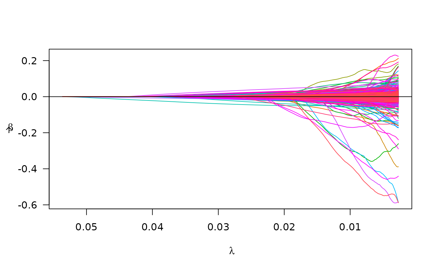
Cross validation
To choose a tuning parameter for a model, plmmr offers a
cross validation method:
cv_fit <- cv_plmm(design = pen_design,
                  type = "blup",
                  return_fit = TRUE,
                  trace = TRUE)
#> Note: The design matrix is being returned as a file-backed big.matrix object -- see bigmemory::big.matrix() documentation for details.
#> Reminder: the X that is returned here is column-standardized
#> Starting decomposition.
#> Calculating the eigendecomposition of K
#> Beginning rotation ('preconditioning').
#> Rotation (preconditioning) finished at  2026-07-01 15:18:18
#> Setting up lambda/preparing for model fitting.
#> Beginning model fitting.
#> Model fitting finished at  2026-07-01 15:18:21
#> 'Fold' argument is either NULL or missing; assigning folds randomly (by default).
#>
#> To specify folds for each observation, supply a vector with fold assignments.
#>
#> Starting cross validation
#> Beginning eigendecomposition in fold  1 :
#> Starting decomposition.
#> Calculating the eigendecomposition of K
#> ** Fitting model in fold 1
#> Beginning rotation ('preconditioning').
#> Rotation (preconditioning) finished at  2026-07-01 15:18:21
#> Beginning model fitting.
#> Model fitting finished at  2026-07-01 15:18:24
#> Beginning eigendecomposition in fold  2 :
#> Starting decomposition.
#> Calculating the eigendecomposition of K
#> ** Fitting model in fold 2
#> Beginning rotation ('preconditioning').
#> Rotation (preconditioning) finished at  2026-07-01 15:18:25
#> Beginning model fitting.
#> Model fitting finished at  2026-07-01 15:18:27
#> Beginning eigendecomposition in fold  3 :
#> Starting decomposition.
#> Calculating the eigendecomposition of K
#> ** Fitting model in fold 3
#> Beginning rotation ('preconditioning').
#> Rotation (preconditioning) finished at  2026-07-01 15:18:28
#> Beginning model fitting.
#> Model fitting finished at  2026-07-01 15:18:30
#> Beginning eigendecomposition in fold  4 :
#> Starting decomposition.
#> Calculating the eigendecomposition of K
#> ** Fitting model in fold 4
#> Beginning rotation ('preconditioning').
#> Rotation (preconditioning) finished at  2026-07-01 15:18:31
#> Beginning model fitting.
#> Model fitting finished at  2026-07-01 15:18:33
#> Beginning eigendecomposition in fold  5 :
#> Starting decomposition.
#> Calculating the eigendecomposition of K
#> ** Fitting model in fold 5
#> Beginning rotation ('preconditioning').
#> Rotation (preconditioning) finished at  2026-07-01 15:18:34
#> Beginning model fitting.
#> Model fitting finished at  2026-07-01 15:18:36
There are plot and summary methods for CV models as well:
summary(cv_fit) # summary at lambda value that minimizes CV error
#> lasso-penalized model with n=1401 and p=4370
#> At minimum cross-validation error (lambda=0.0426):
#> -------------------------------------------------
#>   Nonzero coefficients: 3
#>   Cross-validation error (deviance): 0.17
#>   Scale estimate (sigma): 0.417
plot(cv_fit)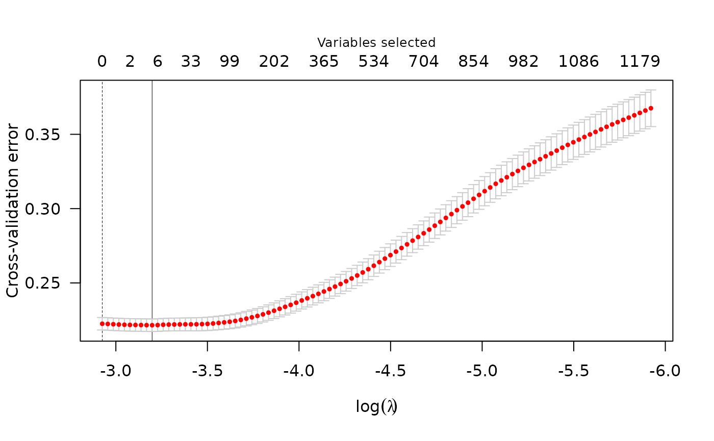
Details: create_design() for PLINK data
The call to create_design() involves these steps:
Integrate in the external phenotype information, if supplied. Note: Any samples in the PLINK data that do not have a phenotype value in the specified additional phenotype file will be removed from the analysis.
Identify missing values in both samples and SNPs/features.
Impute missing values per user’s specified method. See R documentation for
bigsnpr::snp_fastImputeSimple()for more details. Note: the plmmr package cannot fit models if datasets have missing values. All missing values must be imputed or subset out before analysis.Integrate in the external predictor information, if supplied. This could be a matrix of meta-data (e.g., age, principal components, etc.). Note: If there are samples in the supplied file that are not included in the PLINK data, these will be removed. For example, if you have more phenotyped participants than genotyped participants in your study,
plmmr::create_design()will create a matrix of data representing all the genotyped samples that also have data in the supplied external phenotype file.Create a design matrix that represents the nonsingular features and the samples that have predictor and phenotype information available (in the case where external data are supplied).
Standardize the design matrix so that all columns have mean of 0 and variance of 1.